Mathematics

Multivariable Calculus and Vector Analysis

English · 85 pp. PDF

About these notes. These are English notes for the Calculus III (Multivariable Calculus). They follow a Chapter–Lesson–Subsection hierarchy and blend rigorous statements and proofs with geometric intuition, worked examples, and short exercises. The emphasis is on building reliable computational skills (partial derivatives, multiple integrals, coordinate changes) while also clarifying the underlying ideas (linearization, optimization, flux/circulation, and the major integral theorems). Whenever a formula appears, the goal is not only to use it correctly, but also to understand why it is true and when it is the right tool.

1 Chapter 1: Vectors and the Geometry of Space

Key Idea

Multivariable Calculus is built on geometry in $\mathbb{R}^2$ and $\mathbb{R}^3$. Vectors encode direction and magnitude, dot products measure alignment, cross products encode oriented area and normals, and lines/planes give the basic language for geometry in space.

1.1 Lesson 1.1: Vectors in Two and Three Dimensions

1.1.1 Scalars and Vectors

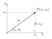
Definition 1.1 (Scalar vs. Vector). A scalar is a real number (e.g., temperature, mass, time). A vector is a quantity with both magnitude and direction. In $\mathbb{R}^2$ or $\mathbb{R}^3$, vectors are typically written in component form: \[\boldsymbol{v}=\langle v_1,v_2\rangle \in \mathbb{R}^2, \qquad \boldsymbol{v}=\langle v_1,v_2,v_3\rangle \in \mathbb{R}^3.\]

Remark 2 (Two equivalent viewpoints). A vector can be viewed as (i) a directed line segment (free to slide without changing the vector), or (ii) a coordinate tuple. The geometry is the reason vectors matter; the coordinates are how we compute.

1.1.2 Geometric Interpretation and Component Form

Definition 1.3 (Position vector and displacement). If $P=(x_1,y_1,z_1)$ and $Q=(x_2,y_2,z_2)$ in $\mathbb{R}^3$, the displacement vector from $P$ to $Q$ is \[\overrightarrow{PQ}=\langle x_2-x_1,\; y_2-y_1,\; z_2-z_1\rangle.\] When $P=(0,0,0)$, the vector $\overrightarrow{OQ}$ is called the position vector of $Q$.

A vector $\boldsymbol{v}=\langle v_1,v_2\rangle$ in $\mathbb{R}^2$ and its components.

1.1.3 Magnitude, Distance, and Unit Vectors

Definition 1.4 (Magnitude (length)). For $\boldsymbol{v}=\langle v_1,v_2,v_3\rangle \in \mathbb{R}^3$, the magnitude is \[\begin{equation} \left\lVert \boldsymbol{v}\right\rVert=\sqrt{v_1^2+v_2^2+v_3^2}. \end{equation}\] In $\mathbb{R}^2$ the same formula holds without the $v_3$ term.

Proposition 1.5 (Distance formula). For points $P,Q\in \mathbb{R}^n$, the distance is \[d(P,Q)=\left\lVert \overrightarrow{PQ}\right\rVert.\]

Definition 1.6 (Unit vector). If $\boldsymbol{v}\neq \boldsymbol{0}$, the unit vector in the direction of $\boldsymbol{v}$ is \[\begin{equation} \hat{\boldsymbol{v}}=\frac{\boldsymbol{v}}{\left\lVert \boldsymbol{v}\right\rVert}. \end{equation}\]

Example 1.7 (Displacement, length, and direction). Let $P=(1,-2,3)$ and $Q=(4,2,1)$. Then \[\overrightarrow{PQ}=\langle 4-1,\;2-(-2),\;1-3\rangle=\langle 3,4,-2\rangle.\] Its length is $\left\lVert \overrightarrow{PQ}\right\rVert=\sqrt{3^2+4^2+(-2)^2}=\sqrt{29}$, and the unit direction is \[\widehat{\overrightarrow{PQ}}=\frac{1}{\sqrt{29}}\langle 3,4,-2\rangle.\]

1.1.4 Standard Basis and Direction Cosines

Definition 1.8 (Standard basis). In $\mathbb{R}^3$, the standard basis vectors are \[\boldsymbol{e}_1=\langle 1,0,0\rangle,\quad \boldsymbol{e}_2=\langle 0,1,0\rangle,\quad \boldsymbol{e}_3=\langle 0,0,1\rangle.\] Any $\boldsymbol{v}=\langle v_1,v_2,v_3\rangle$ can be written as $\boldsymbol{v}=v_1\boldsymbol{e}_1+v_2\boldsymbol{e}_2+v_3\boldsymbol{e}_3$.

Definition 1.9 (Direction angles and direction cosines). Let $\boldsymbol{v}=\langle a,b,c\rangle\neq \boldsymbol{0}$ in $\mathbb{R}^3$. The direction angles $\alpha,\beta,\gamma$ are the angles between $\boldsymbol{v}$ and the positive $x$-, $y$-, $z$-axes respectively. The direction cosines are \[\begin{equation} \cos\alpha=\frac{a}{\left\lVert \boldsymbol{v}\right\rVert},\qquad \cos\beta=\frac{b}{\left\lVert \boldsymbol{v}\right\rVert},\qquad \cos\gamma=\frac{c}{\left\lVert \boldsymbol{v}\right\rVert}. \end{equation}\] They satisfy $\cos^2\alpha+\cos^2\beta+\cos^2\gamma=1$.

Exercise 1.10. Let $\boldsymbol{v}=\langle -2,1,2\rangle$.

Compute $\left\lVert \boldsymbol{v}\right\rVert$ and $\hat{\boldsymbol{v}}$.
Compute the direction cosines.

1.2 Lesson 1.2: Vector Operations

1.2.1 Addition, Subtraction, and Scalar Multiplication

Definition 1.11 (Algebraic operations). For $\boldsymbol{u}=\langle u_1,u_2,u_3\rangle$ and $\boldsymbol{v}=\langle v_1,v_2,v_3\rangle$ in $\mathbb{R}^3$ and scalar $c\in\mathbb{R}$: \[\boldsymbol{u}+\boldsymbol{v}=\langle u_1+v_1,\;u_2+v_2,\;u_3+v_3\rangle,\qquad \boldsymbol{u}-\boldsymbol{v}=\langle u_1-v_1,\;u_2-v_2,\;u_3-v_3\rangle,\] \[c\boldsymbol{v}=\langle cv_1,\;cv_2,\;cv_3\rangle.\] (Identical formulas hold in $\mathbb{R}^2$.)

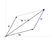
Vector addition via the head-to-tail rule / parallelogram rule.

Remark 12 (Geometric meaning). $\boldsymbol{u}+\boldsymbol{v}$ means: start at the tail of $\boldsymbol{u}$, walk to its head, then place $\boldsymbol{v}$ at that head and walk again. The overall displacement is the sum.

1.2.2 Linear Combinations and Span

Definition 1.13 (Linear combination). A vector of the form $a\boldsymbol{u}+b\boldsymbol{v}$ (with scalars $a,b\in\mathbb{R}$) is called a linear combination of $\boldsymbol{u}$ and $\boldsymbol{v}$.

Key Idea

Thinking in linear combinations is the bridge from geometry to computation: choose convenient vectors, then express what you need as a combination of them.

Example 1.14 (Midpoint formula as a vector statement). Let $A,B\in\mathbb{R}^n$ with position vectors $\boldsymbol{a},\boldsymbol{b}$. The midpoint $M$ of segment $AB$ has position vector \[\boldsymbol{m}=\frac{\boldsymbol{a}+\boldsymbol{b}}{2}.\] Reason: from $A$, moving halfway toward $B$ means adding $\tfrac12(\boldsymbol{b}-\boldsymbol{a})$: $\boldsymbol{m}=\boldsymbol{a}+\tfrac12(\boldsymbol{b}-\boldsymbol{a})=\tfrac12(\boldsymbol{a}+\boldsymbol{b})$.

1.2.3 Basic Vector Identities

Proposition 1.15 (Core identities). For vectors $\boldsymbol{u},\boldsymbol{v},\boldsymbol{w}$ and scalar $c$: \[\boldsymbol{u}+\boldsymbol{v}=\boldsymbol{v}+\boldsymbol{u},\quad (\boldsymbol{u}+\boldsymbol{v})+\boldsymbol{w}=\boldsymbol{u}+(\boldsymbol{v}+\boldsymbol{w}),\quad c(\boldsymbol{u}+\boldsymbol{v})=c\boldsymbol{u}+c\boldsymbol{v},\] \[(c+d)\boldsymbol{v}=c\boldsymbol{v}+d\boldsymbol{v},\quad c(d\boldsymbol{v})=(cd)\boldsymbol{v},\quad 1\cdot\boldsymbol{v}=\boldsymbol{v},\quad 0\cdot\boldsymbol{v}=\boldsymbol{0}.\]

Exercise 1.16. Let $\boldsymbol{u}=\langle 1,-2,0\rangle$ and $\boldsymbol{v}=\langle 3,1,4\rangle$.

Compute $\boldsymbol{u}+2\boldsymbol{v}$ and $\boldsymbol{v}-\boldsymbol{u}$.
Find scalars $a,b$ such that $a\boldsymbol{u}+b\boldsymbol{v}=\langle 7,0,8\rangle$ (if possible).

1.3 Lesson 1.3: The Dot Product

1.3.1 Definition and Algebraic Properties

Definition 1.17 (Dot product). For $\boldsymbol{a}=\langle a_1,\dots,a_n\rangle$ and $\boldsymbol{b}=\langle b_1,\dots,b_n\rangle$ in $\mathbb{R}^n$, the dot product is \[\begin{equation} \boldsymbol{a}\cdot\boldsymbol{b}=\sum_{i=1}^n a_i b_i. \end{equation}\]

Proposition 1.18 (Basic properties). For $\boldsymbol{a},\boldsymbol{b},\boldsymbol{c}\in\mathbb{R}^n$ and $k\in\mathbb{R}$: \[\boldsymbol{a}\cdot\boldsymbol{b}=\boldsymbol{b}\cdot\boldsymbol{a},\quad (\boldsymbol{a}+\boldsymbol{b})\cdot\boldsymbol{c}=\boldsymbol{a}\cdot\boldsymbol{c}+\boldsymbol{b}\cdot\boldsymbol{c},\quad (k\boldsymbol{a})\cdot\boldsymbol{b}=k(\boldsymbol{a}\cdot\boldsymbol{b}).\] Also $\boldsymbol{a}\cdot\boldsymbol{a}\ge 0$ with equality iff $\boldsymbol{a}=\boldsymbol{0}$.

Remark 19 (Length from dot product). From Definition 1.17, we get $\left\lVert \boldsymbol{a}\right\rVert=\sqrt{\boldsymbol{a}\cdot\boldsymbol{a}}$, consistent with Definition 1.4.

1.3.2 Geometric Interpretation, Angles, and Orthogonality

Theorem 1.20 (Dot product and angle). For nonzero vectors $\boldsymbol{a},\boldsymbol{b}\in\mathbb{R}^n$, the angle $\theta\in[0,\pi]$ between them satisfies \[\begin{equation} \boldsymbol{a}\cdot\boldsymbol{b}=\left\lVert \boldsymbol{a}\right\rVert\;\left\lVert \boldsymbol{b}\right\rVert\cos\theta. \end{equation}\]

Definition 1.21 (Orthogonality). Vectors $\boldsymbol{a}$ and $\boldsymbol{b}$ are orthogonal (perpendicular) if $\boldsymbol{a}\cdot\boldsymbol{b}=0$.

1.3.3 Projections

Definition 1.22 (Vector projection). For $\boldsymbol{b}\neq\boldsymbol{0}$, the projection of $\boldsymbol{a}$ onto $\boldsymbol{b}$ is \[\begin{equation} \operatorname{proj}_{\boldsymbol{b}}(\boldsymbol{a}) =\left(\frac{\boldsymbol{a}\cdot\boldsymbol{b}}{\left\lVert \boldsymbol{b}\right\rVert^2}\right)\boldsymbol{b}. \end{equation}\] The scalar projection (signed length) is $\operatorname{comp}_{\boldsymbol{b}}(\boldsymbol{a})=\dfrac{\boldsymbol{a}\cdot\boldsymbol{b}}{\left\lVert \boldsymbol{b}\right\rVert}$.

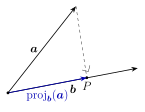
Projection of $\boldsymbol{a}$ onto $\boldsymbol{b}$: the shadow of $\boldsymbol{a}$ along the direction of $\boldsymbol{b}$.

Example 1.23 (Angle and projection). Let $\boldsymbol{a}=\langle 1,2,2\rangle$ and $\boldsymbol{b}=\langle 2,1,-2\rangle$. \[\boldsymbol{a}\cdot\boldsymbol{b}=1\cdot 2+2\cdot 1+2\cdot(-2)=2+2-4=0,\] so $\boldsymbol{a}\perp\boldsymbol{b}$. Therefore the projection in Definition 1.22 is $\operatorname{proj}_{\boldsymbol{b}}(\boldsymbol{a})=\boldsymbol{0}$.

Exercise 1.24. A force $\boldsymbol{F}=\langle 10,0,0\rangle$ moves an object along displacement $\boldsymbol{d}=\langle 3,4,0\rangle$. Compute the work $W=\boldsymbol{F}\cdot\boldsymbol{d}$ and interpret it geometrically via Theorem 1.20.

1.4 Lesson 1.4: The Cross Product

1.4.1 Definition and Computation

Definition 1.25 (Cross product in $\mathbb{R}^3$). For $\boldsymbol{a}=\langle a_1,a_2,a_3\rangle$ and $\boldsymbol{b}=\langle b_1,b_2,b_3\rangle$ in $\mathbb{R}^3$, the cross product is \[\begin{equation} \boldsymbol{a}\times\boldsymbol{b} = \left\langle a_2b_3-a_3b_2,\; a_3b_1-a_1b_3,\; a_1b_2-a_2b_1 \right\rangle. \end{equation}\]

Proposition 1.26 (Algebraic properties). For $\boldsymbol{a},\boldsymbol{b},\boldsymbol{c}\in\mathbb{R}^3$ and $k\in\mathbb{R}$: \[\boldsymbol{a}\times\boldsymbol{b}=-(\boldsymbol{b}\times\boldsymbol{a}),\qquad (\boldsymbol{a}+\boldsymbol{b})\times\boldsymbol{c}=\boldsymbol{a}\times\boldsymbol{c}+\boldsymbol{b}\times\boldsymbol{c},\qquad (k\boldsymbol{a})\times\boldsymbol{b}=k(\boldsymbol{a}\times\boldsymbol{b}),\] and $\boldsymbol{a}\times\boldsymbol{a}=\boldsymbol{0}$.

1.4.2 Geometry: Orientation and Area

Theorem 1.27 (Magnitude and geometric meaning). If $\theta$ is the angle between nonzero $\boldsymbol{a},\boldsymbol{b}\in\mathbb{R}^3$, then \[\begin{equation} \left\lVert \boldsymbol{a}\times\boldsymbol{b}\right\rVert=\left\lVert \boldsymbol{a}\right\rVert\;\left\lVert \boldsymbol{b}\right\rVert\sin\theta. \end{equation}\] Moreover, $\boldsymbol{a}\times\boldsymbol{b}$ is perpendicular to both $\boldsymbol{a}$ and $\boldsymbol{b}$, with direction determined by the right-hand rule.

Key Idea

Dot product measures alignment (via $\cos\theta$). Cross product measures perpendicular area (via $\sin\theta$) and produces a normal direction.

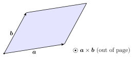
The area of the parallelogram spanned by $\boldsymbol{a}$ and $\boldsymbol{b}$ equals $\left\lVert \boldsymbol{a}\times\boldsymbol{b}\right\rVert$.

Corollary 1.28 (Areas). The area of the parallelogram spanned by $\boldsymbol{a},\boldsymbol{b}$ is $\left\lVert \boldsymbol{a}\times\boldsymbol{b}\right\rVert$, and the area of the triangle spanned by them is $\tfrac12\left\lVert \boldsymbol{a}\times\boldsymbol{b}\right\rVert$.

Example 1.29 (Area of a triangle from three points). Let $A=(1,0,0)$, $B=(2,1,0)$, and $C=(0,2,1)$. Then \[\overrightarrow{AB}=\langle 1,1,0\rangle,\qquad \overrightarrow{AC}=\langle -1,2,1\rangle.\] Compute \[\overrightarrow{AB}\times\overrightarrow{AC} = \langle 1\cdot 1-0\cdot 2,\; 0\cdot(-1)-1\cdot 1,\; 1\cdot 2-1\cdot(-1)\rangle = \langle 1,-1,3\rangle.\] So $\left\lVert \overrightarrow{AB}\times\overrightarrow{AC}\right\rVert=\sqrt{1^2+(-1)^2+3^2}=\sqrt{11}$, and the triangle area is $\dfrac12\sqrt{11}$.

Exercise 1.30. Find a nonzero normal vector to the plane through $P=(1,0,2)$, $Q=(2,1,2)$, and $R=(0,2,3)$ using a cross product.

1.5 Lesson 1.5: Lines and Planes in Space

1.5.1 Vector and Parametric Equations of Lines

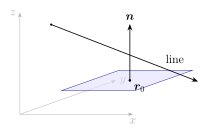
Definition 1.31 (Line in $\mathbb{R}^3$). A line through a point with position vector $\boldsymbol{r}_0$ and direction vector $\boldsymbol{v}\neq \boldsymbol{0}$ has vector equation \[\begin{equation} \boldsymbol{r}(t)=\boldsymbol{r}_0+t\boldsymbol{v},\qquad t\in\mathbb{R}. \end{equation}\] If $\boldsymbol{r}=\langle x,y,z\rangle$, $\boldsymbol{r}_0=\langle x_0,y_0,z_0\rangle$, and $\boldsymbol{v}=\langle a,b,c\rangle$, then Definition 1.31 is equivalent to the parametric equations \[\begin{equation} x=x_0+at,\qquad y=y_0+bt,\qquad z=z_0+ct. \end{equation}\]

Example 1.32 (Line through two points). The line through $P=(1,2,0)$ and $Q=(4,0,3)$ has direction $\overrightarrow{PQ}=\langle 3,-2,3\rangle$, hence \[\boldsymbol{r}(t)=\langle 1,2,0\rangle+t\langle 3,-2,3\rangle.\]

1.5.2 Equations of Planes

Definition 1.33 (Plane (point-normal form)). A plane through $\boldsymbol{r}_0$ with normal vector $\boldsymbol{n}\neq \boldsymbol{0}$ is the set of points $\boldsymbol{r}$ satisfying \[\begin{equation} \boldsymbol{n}\cdot(\boldsymbol{r}-\boldsymbol{r}_0)=0. \end{equation}\]

Remark 34 (From point-normal to $ax+by+cz=d$). If $\boldsymbol{n}=\langle a,b,c\rangle$ and $\boldsymbol{r}=\langle x,y,z\rangle$, then Definition 1.33 becomes \[a(x-x_0)+b(y-y_0)+c(z-z_0)=0 \quad\Longleftrightarrow\quad ax+by+cz=d,\ \ d=ax_0+by_0+cz_0.\]

A plane with normal vector $\boldsymbol{n}$ and a line in space.

1.5.3 Distances Between Points, Lines, and Planes

Proposition 1.35 (Distance from a point to a plane). For a plane $ax+by+cz=d$ and point $P=(x_0,y_0,z_0)$, the distance is \[\begin{equation} \operatorname{dist}(P,\Pi)=\frac{|ax_0+by_0+cz_0-d|}{\sqrt{a^2+b^2+c^2}}. \end{equation}\]

Remark 36 (Why the formula is reasonable). The numerator is the signed “how much the plane equation fails” at $P$. Dividing by $\sqrt{a^2+b^2+c^2}=\left\lVert \langle a,b,c\rangle\right\rVert$ rescales that failure into an actual geometric distance along the normal direction.

Proposition 1.37 (Distance from a point to a line in $\mathbb{R}^3$). Let a line be $\boldsymbol{r}(t)=\boldsymbol{r}_0+t\boldsymbol{v}$ with $\boldsymbol{v}\neq \boldsymbol{0}$. For a point with position vector $\boldsymbol{p}$, \[\begin{equation} \operatorname{dist}(P,\ell)=\frac{\left\lVert (\boldsymbol{p}-\boldsymbol{r}_0)\times\boldsymbol{v}\right\rVert}{\left\lVert \boldsymbol{v}\right\rVert}. \end{equation}\]

Example 1.38 (Point-to-plane distance). Find the distance from $P=(1,2,3)$ to the plane $2x-y+2z=5$. Using Proposition 1.35 with $(a,b,c,d)=(2,-1,2,5)$: \[\operatorname{dist}(P,\Pi)=\frac{|2(1)-1(2)+2(3)-5|}{\sqrt{2^2+(-1)^2+2^2}} =\frac{|2-2+6-5|}{\sqrt{9}} =\frac{1}{3}.\]

Example 1.39 (Plane through three points). Find an equation for the plane through $A=(1,0,2)$, $B=(2,1,2)$, $C=(0,2,3)$. Compute direction vectors \[\overrightarrow{AB}=\langle 1,1,0\rangle,\qquad \overrightarrow{AC}=\langle -1,2,1\rangle,\] so a normal is \[\boldsymbol{n}=\overrightarrow{AB}\times\overrightarrow{AC}=\langle 1,-1,3\rangle\] (as in a previous computation pattern). Using point-normal form Definition 1.33 with $\boldsymbol{r}_0=\langle 1,0,2\rangle$: \[\langle 1,-1,3\rangle\cdot\langle x-1,\ y-0,\ z-2\rangle=0\] \[(x-1)-y+3(z-2)=0 \quad\Longleftrightarrow\quad x-y+3z=7.\]

Exercise 1.40. A line is given by $\boldsymbol{r}(t)=\langle 1,0,1\rangle+t\langle 2,-1,2\rangle$.

Determine whether the line is parallel to the plane $2x+y-2z=3$.
Compute the distance from $P=(0,1,0)$ to the line using Proposition 1.37.

Chapter 1 Checklist

Convert between points and displacement vectors; compute lengths and unit vectors Definitions 1.4 and 1.6.
Compute dot products; use them for angles and projections Theorem 1.20 and Definition 1.22.
Compute cross products; use them for normals and areas Definition 1.25 and Theorem 1.27.
Write lines and planes in vector/parametric/normal forms Definitions 1.31 and 1.33.
Use projection-based distance formulas to lines/planes Propositions 1.35 and 1.37.

2 Chapter 2: Vector-Valued Functions and Space Curves

Key Idea

A vector-valued function $\boldsymbol{r}(t)$ packages several scalar functions into one object. Geometrically, it traces a parametrized curve in space. Once you accept “differentiate and integrate componentwise,” the calculus becomes familiar; the new content is the geometry: tangent vectors, speed, arc length, curvature, and how acceleration splits into tangential/normal parts.

2.1 Lesson 2.1: Vector-Valued Functions

2.1.1 Definitions and Examples

Definition 2.1 (Vector-valued function). A vector-valued function is a function \[\boldsymbol{r}:I\subset\mathbb{R}\to \mathbb{R}^n,\qquad \boldsymbol{r}(t)=\langle f_1(t),f_2(t),\dots,f_n(t)\rangle,\] where each $f_i$ is a scalar function on $I$. When $n=2$ or $3$, $\boldsymbol{r}(t)$ defines a parametric curve in the plane or in space.

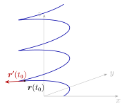
Example 2.2 (A standard space curve: helix). \[\boldsymbol{r}(t)=\langle \cos t,\ \sin t,\ t\rangle,\qquad t\in[0,4\pi].\] As $t$ increases, $(\cos t,\sin t)$ runs around the unit circle while $z=t$ rises linearly, forming a helix.

Remark 43 (Most intuitive interpretation). Think of $t$ as “time.” Then $\boldsymbol{r}(t)$ is the position of a particle at time $t$. This viewpoint turns derivatives into velocity/acceleration automatically.

2.1.2 Limits and Continuity

Definition 2.4 (Limit of a vector-valued function). Let $\boldsymbol{r}(t)=\langle f_1(t),\dots,f_n(t)\rangle$. We say \[\lim_{t\to a}\boldsymbol{r}(t)=\boldsymbol{L}=\langle L_1,\dots,L_n\rangle\] if and only if $\lim_{t\to a} f_i(t)=L_i$ for every component $i=1,\dots,n$.

Proposition 2.5 (Continuity). $\boldsymbol{r}$ is continuous at $t=a$ if and only if each component $f_i$ is continuous at $a$.

Example 2.6 (Componentwise limit). Let $\boldsymbol{r}(t)=\langle t^2,\ \sin t,\ e^t\rangle$. Then \[\lim_{t\to 0}\boldsymbol{r}(t)=\langle 0,\ 0,\ 1\rangle.\]

2.1.3 Graphs of Vector-Valued Functions (Parametric Curves)

Definition 2.7 (Parameter and trace). The graph of $\boldsymbol{r}(t)$ (often called its trace) is the set of points in $\mathbb{R}^n$: \[\{\boldsymbol{r}(t): t\in I\}.\] Changing the parameterization can trace the same geometric curve with different speed or orientation.

A space curve (helix) traced by a vector-valued function, with a tangent (velocity) vector at $t_0$.

Exercise 2.8. Give two different parameterizations of the line segment from $A=(0,0,0)$ to $B=(2,1,3)$. (Hint: one can trace it in 1 second, another in 5 seconds.)

2.2 Lesson 2.2: Derivatives of Vector-Valued Functions

2.2.1 Componentwise Differentiation

Definition 2.9 (Derivative). Let $\boldsymbol{r}(t)=\langle f_1(t),\dots,f_n(t)\rangle$. If each $f_i'(t)$ exists, define \[\boldsymbol{r}'(t)=\left\langle f_1'(t),f_2'(t),\dots,f_n'(t)\right\rangle.\]

Proposition 2.10 (Derivative rules). All standard rules apply componentwise: linearity, product rules for scalar multiples, and chain rule for each component.

2.2.2 Velocity and Acceleration Vectors

Definition 2.11 (Kinematics in vector form). If $\boldsymbol{r}(t)$ is a position vector in $\mathbb{R}^3$, then \[\boldsymbol{v}(t)=\boldsymbol{r}'(t)\quad \text{(velocity)},\qquad \boldsymbol{a}(t)=\boldsymbol{r}''(t)\quad \text{(acceleration)}.\] The speed is the scalar $\left\lVert \boldsymbol{v}(t)\right\rVert$.

Remark 52 (Plain-language meaning). $\boldsymbol{v}(t)$ points in the direction of motion; its length is “how fast.” $\boldsymbol{a}(t)$ measures how velocity changes: it captures both speeding up/slowing down and turning.

2.2.3 Tangent Vectors and Tangent Lines

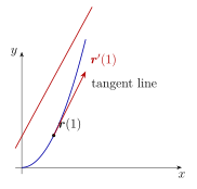
Definition 2.13 (Tangent line). If $\boldsymbol{r}$ is differentiable at $t=t_0$ and $\boldsymbol{r}'(t_0)\neq\boldsymbol{0}$, the tangent line at $t_0$ is \[\ell:\ \boldsymbol{\ell}(s)=\boldsymbol{r}(t_0)+s\,\boldsymbol{r}'(t_0),\qquad s\in\mathbb{R}.\] (Using $s$ avoids confusion with the original parameter $t$.)

Example 2.14 (Differentiate and form a tangent line). Let $\boldsymbol{r}(t)=\langle \cos t,\ \sin t,\ t\rangle$. Then \[\boldsymbol{r}'(t)=\langle -\sin t,\ \cos t,\ 1\rangle,\qquad \boldsymbol{r}''(t)=\langle -\cos t,\ -\sin t,\ 0\rangle.\] At $t_0=0$, \[\boldsymbol{r}(0)=\langle 1,0,0\rangle,\qquad \boldsymbol{r}'(0)=\langle 0,1,1\rangle,\] so the tangent line is $\boldsymbol{\ell}(s)=\langle 1,0,0\rangle+s\langle 0,1,1\rangle$.

Planar parametric curve $\boldsymbol{r}(t)=\langle t,t^2\rangle$ with tangent vector and tangent line at $t_0=1$.

Exercise 2.15. Let $\boldsymbol{r}(t)=\langle e^t,\ t^2,\ \ln(1+t)\rangle$ (domain $t>-1$). Compute $\boldsymbol{r}'(t)$ and the tangent line at $t_0=0$.

2.3 Lesson 2.3: Integrals of Vector-Valued Functions

2.3.1 Antiderivatives

Definition 2.16 (Indefinite integral). If $\boldsymbol{r}(t)=\langle f(t),g(t),h(t)\rangle$ is continuous, define \[\int \boldsymbol{r}(t)\,dt = \left\langle \int f(t)\,dt,\ \int g(t)\,dt,\ \int h(t)\,dt \right\rangle = \boldsymbol{R}(t)+\boldsymbol{C},\] where $\boldsymbol{R}'(t)=\boldsymbol{r}(t)$ and $\boldsymbol{C}$ is a constant vector.

Proposition 2.17 (Fundamental Theorem (vector form)). If $\boldsymbol{r}$ is continuous on $[a,b]$ and $\boldsymbol{R}'(t)=\boldsymbol{r}(t)$, then \[\int_a^b \boldsymbol{r}(t)\,dt=\boldsymbol{R}(b)-\boldsymbol{R}(a).\]

2.3.2 Definite Integrals

Definition 2.18 (Definite integral). For continuous $\boldsymbol{r}(t)=\langle f_1(t),\dots,f_n(t)\rangle$, \[\int_a^b \boldsymbol{r}(t)\,dt = \left\langle \int_a^b f_1(t)\,dt,\ \dots,\ \int_a^b f_n(t)\,dt\right\rangle.\]

2.3.3 Applications to Motion

Proposition 2.19 (Displacement from velocity). If $\boldsymbol{v}(t)=\boldsymbol{r}'(t)$, then \[\boldsymbol{r}(b)-\boldsymbol{r}(a)=\int_a^b \boldsymbol{v}(t)\,dt.\]

Remark 60 (Displacement vs. distance traveled). Displacement is the net change in position: $\boldsymbol{r}(b)-\boldsymbol{r}(a)$. Total distance traveled is \[\int_a^b \left\lVert \boldsymbol{v}(t)\right\rVert\,dt,\] which is generally larger (unless you move without reversing/turning).

Example 2.21 (Displacement and distance). Let $\boldsymbol{v}(t)=\langle 1,\ 2t,\ 0\rangle$ for $t\in[0,2]$, and $\boldsymbol{r}(0)=\langle 0,0,0\rangle$. Then \[\boldsymbol{r}(t)=\int_0^t \boldsymbol{v}(s)\,ds = \left\langle \int_0^t 1\,ds,\ \int_0^t 2s\,ds,\ 0\right\rangle = \langle t,\ t^2,\ 0\rangle.\] So displacement on $[0,2]$ is $\boldsymbol{r}(2)-\boldsymbol{r}(0)=\langle 2,4,0\rangle$. Distance traveled is \[\int_0^2 \left\lVert \boldsymbol{v}(t)\right\rVert\,dt=\int_0^2 \sqrt{1+(2t)^2}\,dt.\] (Closed form exists, but the key point is the setup: distance uses speed $\left\lVert \boldsymbol{v}\right\rVert$.)

Exercise 2.22. Suppose $\boldsymbol{a}(t)=\langle 0,-g,0\rangle$ with constant $g>0$, and $\boldsymbol{v}(0)=\langle v_0,0,0\rangle$, $\boldsymbol{r}(0)=\langle 0,0,0\rangle$. Find $\boldsymbol{v}(t)$ and $\boldsymbol{r}(t)$.

2.4 Lesson 2.4: Arc Length and Curvature

2.4.1 Arc Length of Space Curves

Theorem 2.23 (Arc length formula). If $\boldsymbol{r}:[a,b]\to\mathbb{R}^3$ is continuously differentiable, then the arc length of its trace is \[\begin{equation} L=\int_a^b \left\lVert \boldsymbol{r}'(t)\right\rVert\,dt. \end{equation}\]

Remark 64 (Intuition in one sentence). Over a tiny time step $\Delta t$, you move about $\left\lVert \boldsymbol{r}'(t)\right\rVert\,\Delta t$; summing these and taking a limit yields Theorem 2.23.

Example 2.25 (Arc length of a helix segment). For $\boldsymbol{r}(t)=\langle \cos t,\ \sin t,\ t\rangle$ on $[0,2\pi]$, \[\boldsymbol{r}'(t)=\langle -\sin t,\ \cos t,\ 1\rangle,\qquad \left\lVert \boldsymbol{r}'(t)\right\rVert=\sqrt{\sin^2 t+\cos^2 t+1}=\sqrt{2}.\] Thus $L=\int_0^{2\pi}\sqrt{2}\,dt=2\pi\sqrt{2}$.

2.4.2 Unit Tangent and Normal Vectors

Definition 2.26 (Unit tangent). If $\boldsymbol{r}'(t)\neq\boldsymbol{0}$, the unit tangent vector is \[\begin{equation} \boldsymbol{T}(t)=\frac{\boldsymbol{r}'(t)}{\left\lVert \boldsymbol{r}'(t)\right\rVert}. \end{equation}\]

Definition 2.27 (Principal normal). If $\boldsymbol{T}'(t)\neq\boldsymbol{0}$, define the principal unit normal vector by \[\boldsymbol{N}(t)=\frac{\boldsymbol{T}'(t)}{\left\lVert \boldsymbol{T}'(t)\right\rVert}.\] In $\mathbb{R}^3$, one also defines the binormal $\boldsymbol{B}(t)=\boldsymbol{T}(t)\times \boldsymbol{N}(t)$.

2.4.3 Curvature of a Curve

Definition 2.28 (Curvature). Let $s$ be arc length (so $ds/dt=\left\lVert \boldsymbol{r}'(t)\right\rVert$). The curvature is \[\kappa=\left\lVert \frac{d\boldsymbol{T}}{ds}\right\rVert.\] Equivalently (as a function of $t$), \[\begin{equation} \kappa(t)=\frac{\left\lVert \boldsymbol{T}'(t)\right\rVert}{\left\lVert \boldsymbol{r}'(t)\right\rVert}. \end{equation}\]

Theorem 2.29 (Cross-product curvature formula). If $\boldsymbol{r}$ is twice differentiable and $\boldsymbol{r}'(t)\neq \boldsymbol{0}$, then \[\begin{equation} \kappa(t)=\frac{\left\lVert \boldsymbol{r}'(t)\times \boldsymbol{r}''(t)\right\rVert}{\left\lVert \boldsymbol{r}'(t)\right\rVert^{3}}. \end{equation}\]

Example 2.30 (Curvature of $\langle \cos t,\sin t,t\rangle$ is constant). For $\boldsymbol{r}(t)=\langle \cos t,\ \sin t,\ t\rangle$: \[\boldsymbol{r}'(t)=\langle -\sin t,\ \cos t,\ 1\rangle,\quad \boldsymbol{r}''(t)=\langle -\cos t,\ -\sin t,\ 0\rangle.\] Compute \[\boldsymbol{r}'(t)\times \boldsymbol{r}''(t) = \left\langle 1\cdot(-\sin t)-1\cdot(-\sin t)?,\ \dots \right\rangle\] Rather than expand blindly, do it carefully: \[\begin{align*} \boldsymbol{r}'(t)\times \boldsymbol{r}''(t) &= \begin{vmatrix} \boldsymbol{i} & \boldsymbol{j} & \boldsymbol{k}\\ -\sin t & \cos t & 1\\ -\cos t & -\sin t & 0 \end{vmatrix} \\ &= \bigl\langle \cos t\cdot 0-1\cdot(-\sin t), \\ &\quad\quad -\bigl((-\sin t)\cdot 0-1\cdot(-\cos t)\bigr), \\ &\quad\quad (-\sin t)(-\sin t)-(\cos t)(-\cos t) \bigr\rangle \end{align*}\] \[=\langle \sin t,\ -\cos t,\ 1\rangle.\] Hence $\left\lVert \boldsymbol{r}'(t)\times \boldsymbol{r}''(t)\right\rVert=\sqrt{\sin^2 t+\cos^2 t+1}=\sqrt{2}$ and $\left\lVert \boldsymbol{r}'(t)\right\rVert=\sqrt{2}$, so by Theorem 2.29, \[\kappa(t)=\frac{\sqrt{2}}{(\sqrt{2})^3}=\frac{1}{2}.\]

Exercise 2.31. For the circle $\boldsymbol{r}(t)=\langle a\cos t,\ a\sin t,\ 0\rangle$ ($a>0$), compute $\kappa(t)$ and interpret the result geometrically.

2.5 Lesson 2.5: Motion in Space

2.5.1 Kinematics in Three Dimensions

Notation 72. We will write $\boldsymbol{v}=\boldsymbol{r}'$ and $\boldsymbol{a}=\boldsymbol{r}''$ as in Definition 2.11, and speed $v=\left\lVert \boldsymbol{v}\right\rVert$ (note: $v$ is a scalar here).

Proposition 2.33 (Decomposition of acceleration). Assume $\boldsymbol{r}'(t)\neq \boldsymbol{0}$. Then acceleration splits into tangential and normal parts: \[\begin{equation} \boldsymbol{a} = a_T\,\boldsymbol{T} + a_N\,\boldsymbol{N}, \end{equation}\] where \[\begin{equation} a_T=\frac{dv}{dt}=\frac{\boldsymbol{v}\cdot \boldsymbol{a}}{\left\lVert \boldsymbol{v}\right\rVert}, \qquad a_N=\kappa v^2=\frac{\left\lVert \boldsymbol{v}\times \boldsymbol{a}\right\rVert}{\left\lVert \boldsymbol{v}\right\rVert}. \end{equation}\]

Remark 74 (What this means in plain terms). $a_T$ measures speeding up or slowing down. $a_N$ measures turning: even if speed is constant ($a_T=0$), you can still have acceleration if the direction changes.

Example 2.35 (Projectile motion (in a plane, written vectorially)). Let $g>0$ and \[\boldsymbol{r}(t)=\langle v_0\cos\theta\; t,\ v_0\sin\theta\; t-\tfrac12 g t^2,\ 0\rangle.\] Then \[\boldsymbol{v}(t)=\langle v_0\cos\theta,\ v_0\sin\theta-gt,\ 0\rangle,\qquad \boldsymbol{a}(t)=\langle 0,\ -g,\ 0\rangle.\] Acceleration is constant and downward, independent of the current velocity.

Example 2.36 (Uniform circular motion and normal acceleration). If $\boldsymbol{r}(t)=\langle a\cos(\omega t),\ a\sin(\omega t),\ 0\rangle$, then \[\boldsymbol{v}(t)=\langle -a\omega\sin(\omega t),\ a\omega\cos(\omega t),\ 0\rangle,\quad v=\left\lVert \boldsymbol{v}\right\rVert=a\omega \ \text{(constant)}.\] Thus $a_T=dv/dt=0$. Nevertheless, \[\boldsymbol{a}(t)=\langle -a\omega^2\cos(\omega t),\ -a\omega^2\sin(\omega t),\ 0\rangle,\] which points toward the center and has magnitude $a\omega^2=\dfrac{v^2}{a}$, matching $a_N=\kappa v^2$ with $\kappa=1/a$.

Exercise 2.37. A particle moves along $\boldsymbol{r}(t)=\langle t,\ \cos t,\ \sin t\rangle$ for $t\ge 0$.

Compute $\boldsymbol{v}(t)$, $\boldsymbol{a}(t)$, and the speed $v(t)$.
Determine whether the speed is constant.
Compute $\kappa(t)$ using Theorem 2.29.

Chapter 2 Checklist

Treat limits/continuity/derivatives/integrals componentwise (Definitions Definitions 2.4, 2.9 and 2.18).
Interpret $\boldsymbol{r}',\boldsymbol{r}''$ as velocity and acceleration; speed is $\left\lVert \boldsymbol{r}'\right\rVert$.
Build tangent lines from $\boldsymbol{r}(t_0)$ and $\boldsymbol{r}'(t_0)$ (Definition 2.13).
Compute arc length via $L=\int \left\lVert \boldsymbol{r}'\right\rVert\,dt$ (Theorem 2.23).
Compute curvature via $\kappa=\left\lVert \boldsymbol{r}'\times \boldsymbol{r}''\right\rVert/\left\lVert \boldsymbol{r}'\right\rVert^3$ (Theorem 2.29).
Decompose acceleration into tangential/normal components (Proposition 2.33).

3 Chapter 3: Functions of Several Variables

Key Idea

A single-variable function $y=f(x)$ lives on a line and draws a curve. A multivariable function $z=f(x,y)$ lives on a region in the plane and draws a surface in space. Because surfaces are hard to “see” directly, we use level sets (contours) and slices (traces) to understand them, and we use partial derivatives to measure how the output changes when we move in chosen directions.

3.1 Lesson 3.1: Functions of Two and Three Variables

3.1.1 Definitions and Examples

Definition 3.1 (Functions of several variables). A function of two variables is a map \[f:D\subset \mathbb{R}^2 \to \mathbb{R},\qquad (x,y)\mapsto f(x,y),\] where $D$ is the domain. A function of three variables is \[f:D\subset \mathbb{R}^3 \to \mathbb{R},\qquad (x,y,z)\mapsto f(x,y,z).\] The range is $\{f(\boldsymbol{x}): \boldsymbol{x}\in D\}$.

Example 3.2 (Domains).

$f(x,y)=\sqrt{1-x^2-y^2}$ has domain $D=\{(x,y):x^2+y^2\le 1\}$ (a closed disk).
$g(x,y)=\dfrac{1}{x^2+y^2}$ has domain $\mathbb{R}^2\setminus\{(0,0)\}$.
$h(x,y,z)=\ln(z-x^2-y^2)$ has domain $\{(x,y,z): z>x^2+y^2\}$.

Remark 80 (A practical rule). Domains are determined by where the formula makes sense: no division by $0$, even roots require nonnegative input, logarithms require positive input, etc.

3.1.2 Graphs and Level Sets

Definition 3.4 (Graph of $z=f(x,y)$). If $f:D\subset\mathbb{R}^2\to\mathbb{R}$, the graph of $f$ is the set \[\{(x,y,z)\in\mathbb{R}^3: (x,y)\in D,\ z=f(x,y)\}.\]

Definition 3.5 (Level curves and level surfaces). For $f(x,y)$, the level curve at height $c$ is \[f(x,y)=c.\] For $F(x,y,z)$, the level surface at level $c$ is \[F(x,y,z)=c.\]

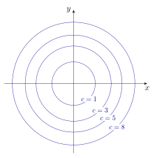
Example 3.6 (A classic: paraboloid and its contours). Let $f(x,y)=x^2+y^2$.

The graph is the paraboloid $z=x^2+y^2$.
The level curves $x^2+y^2=c$ (for $c\ge 0$) are circles of radius $\sqrt{c}$ in the $xy$-plane.

Level curves (contour lines) for $f(x,y)=x^2+y^2$.

3.1.3 Domains and Ranges (Geometric View)

Example 3.7 (Range from geometry). For $f(x,y)=\sqrt{1-x^2-y^2}$ with domain $x^2+y^2\le 1$, we have $0\le 1-x^2-y^2\le 1$, so \[0\le f(x,y)\le 1.\] Geometrically, $z=\sqrt{1-x^2-y^2}$ is the upper hemisphere of the unit sphere, so heights run from $0$ to $1$.

Exercise 3.8. Describe the domain of $f(x,y)=\dfrac{\sqrt{4-x^2}}{y-1}$ and sketch it in the $xy$-plane.

3.2 Lesson 3.2: Limits and Continuity

3.2.1 Limits of Multivariable Functions

Definition 3.9 (Limit in $\mathbb{R}^2$). Let $f:D\subset\mathbb{R}^2\to\mathbb{R}$ and let $(a,b)$ be a limit point of $D$. We say \[\lim_{(x,y)\to(a,b)} f(x,y)=L\] if for every $\varepsilon>0$ there exists $\delta>0$ such that whenever $(x,y)\in D$ and \[0<\sqrt{(x-a)^2+(y-b)^2}<\delta,\] we have $|f(x,y)-L|<\varepsilon$.

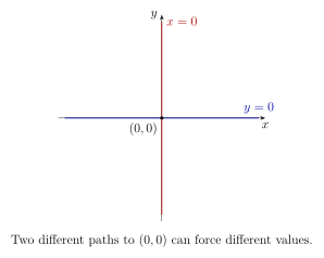
Remark 87 (What changed from Calc I). In one variable, approaching $a$ means coming from the left/right on a line. In two variables, $(x,y)\to(a,b)$ means approaching from infinitely many paths in the plane. This is why limits are harder: you must control all approaches.

3.2.2 When a Limit Does Not Exist

Proposition 3.11 (Path test (useful sufficient test for nonexistence)). If there exist two paths $\gamma_1,\gamma_2$ approaching $(a,b)$ such that \[\lim_{(x,y)\to(a,b)\ \text{along }\gamma_1} f(x,y)\neq \lim_{(x,y)\to(a,b)\ \text{along }\gamma_2} f(x,y),\] then $\lim_{(x,y)\to(a,b)} f(x,y)$ does not exist.

Example 3.12 (Different paths, different limits). Define \[f(x,y)= \begin{cases} \dfrac{x^2-y^2}{x^2+y^2}, & (x,y)\neq(0,0),\\[6pt] 0, & (x,y)=(0,0). \end{cases}\] Along the $x$-axis ($y=0$), for $x\neq 0$, \[f(x,0)=\frac{x^2}{x^2}=1 \quad\Longrightarrow\quad \lim_{x\to 0} f(x,0)=1.\] Along the $y$-axis ($x=0$), for $y\neq 0$, \[f(0,y)=\frac{-y^2}{y^2}=-1 \quad\Longrightarrow\quad \lim_{y\to 0} f(0,y)=-1.\] The two path limits disagree, so the limit at $(0,0)$ does not exist by Proposition 3.11.

Approaching $(0,0)$ along different paths is a standard way to test nonexistence of a limit.

3.2.3 Continuity and Properties

Definition 3.13 (Continuity at a point). A function $f:D\subset\mathbb{R}^2\to\mathbb{R}$ is continuous at $(a,b)\in D$ if \[\lim_{(x,y)\to(a,b)} f(x,y)=f(a,b).\]

Proposition 3.14 (Algebra of continuity). If $f$ and $g$ are continuous at $(a,b)$, then $f+g$, $f-g$, $fg$, and (where defined) $f/g$ are continuous at $(a,b)$. Compositions of continuous functions are continuous.

Remark 92 (A reliable shortcut). Polynomials in $(x,y)$ are continuous everywhere. Rational functions are continuous wherever the denominator is nonzero. Functions built from continuous pieces (roots, trig, exp/log) are continuous where their inputs are valid.

Exercise 3.16. Determine whether $f(x,y)=\dfrac{xy}{x^2+y^2}$ (with $f(0,0)=0$) is continuous at $(0,0)$. (Hint: try the path $y=mx$.)

3.3 Lesson 3.3: Partial Derivatives

3.3.1 Definition of Partial Derivatives

Definition 3.17 (First-order partial derivatives). Let $f(x,y)$ be defined near $(a,b)$. The partial derivatives at $(a,b)$ are \[f_x(a,b)=\lim_{h\to 0}\frac{f(a+h,b)-f(a,b)}{h}, \qquad f_y(a,b)=\lim_{h\to 0}\frac{f(a,b+h)-f(a,b)}{h},\] if the limits exist.

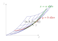
Remark 95 (Plain-language interpretation). $f_x(a,b)$ measures how $f$ changes when you move in the $x$-direction while freezing $y=b$. $f_y(a,b)$ does the same in the $y$-direction while freezing $x=a$. So partial derivatives are “single-variable derivatives of slices.”

3.3.2 Higher-Order Partial Derivatives

Definition 3.19 (Second-order partial derivatives). If $f_x$ and $f_y$ exist near $(a,b)$, we can differentiate again: \[f_{xx}=\frac{\partial}{\partial x}(f_x),\quad f_{yy}=\frac{\partial}{\partial y}(f_y),\quad f_{xy}=\frac{\partial}{\partial y}(f_x),\quad f_{yx}=\frac{\partial}{\partial x}(f_y).\]

3.3.3 Clairaut’s Theorem (Equality of Mixed Partials)

Theorem 3.20 (Clairaut / Schwarz). If $f_{xy}$ and $f_{yx}$ are continuous on an open neighborhood of $(a,b)$, then \[f_{xy}(a,b)=f_{yx}(a,b).\]

Example 3.21 (Computing mixed partials). Let $f(x,y)=x^2y^3+\sin(xy)$. Then \[f_x=2xy^3+y\cos(xy),\qquad f_y=3x^2y^2+x\cos(xy).\] Differentiate again: \[f_{xy}=\frac{\partial}{\partial y}\left(2xy^3+y\cos(xy)\right) =6xy^2+\cos(xy)-xy\sin(xy),\] \[f_{yx}=\frac{\partial}{\partial x}\left(3x^2y^2+x\cos(xy)\right) =6xy^2+\cos(xy)-xy\sin(xy).\] So $f_{xy}=f_{yx}$ (as predicted by Theorem 3.20 since the formula is smooth everywhere).

Partial derivatives come from slopes of slice curves: fix $y=b$ (red) for $f_x$, fix $x=a$ (green) for $f_y$.

Exercise 3.22. Let $f(x,y)=\dfrac{x^2y}{1+y^2}$.

Compute $f_x$ and $f_y$.
Compute $f_{xy}$ and $f_{yx}$ and verify they agree.

3.4 Lesson 3.4: Differentiability and the Gradient

3.4.1 Differentiability

Definition 3.23 (Differentiability in $\mathbb{R}^2$). Let $f$ be defined near $(a,b)$. We say $f$ is differentiable at $(a,b)$ if there exists a linear map \[L(h,k)=Ah+Bk\] such that \[\begin{equation} f(a+h,b+k)=f(a,b)+L(h,k)+o\!\left(\sqrt{h^2+k^2}\right) \quad\text{as }(h,k)\to(0,0). \end{equation}\]

Remark 101 (Why this matters). Differentiability means: near $(a,b)$, the surface is well-approximated by a plane. Continuity alone says “no jumps,” but differentiability says “has a reliable linear approximation.”

Theorem 3.25 (Sufficient condition for differentiability). If $f_x$ and $f_y$ exist in a neighborhood of $(a,b)$ and are continuous at $(a,b)$, then $f$ is differentiable at $(a,b)$.

Proposition 3.26 (Differentiability implies continuity). If $f$ is differentiable at $(a,b)$, then $f$ is continuous at $(a,b)$.

3.4.2 The Gradient Vector

Definition 3.27 (Gradient). If $f:\mathbb{R}^2\to\mathbb{R}$ has partial derivatives, its gradient is \[\nabla f(x,y)=\left\langle f_x(x,y),\, f_y(x,y)\right\rangle.\] More generally for $f:\mathbb{R}^n\to\mathbb{R}$, \[\nabla f=\left\langle \frac{\partial f}{\partial x_1},\dots,\frac{\partial f}{\partial x_n}\right\rangle.\]

Remark 105 (What the gradient “is”). $\nabla f(a,b)$ points in the direction where $f$ increases fastest, and its magnitude is that maximum rate of increase (made precise below).

3.4.3 Directional Derivatives

Definition 3.29 (Directional derivative). Let $\boldsymbol{u}=\langle u_1,u_2\rangle$ be a unit vector. The directional derivative of $f$ at $(a,b)$ in direction $\boldsymbol{u}$ is \[D_{\boldsymbol{u}}f(a,b)=\lim_{h\to 0}\frac{f(a+hu_1,b+hu_2)-f(a,b)}{h},\] if the limit exists.

Theorem 3.30 (Directional derivative via gradient). If $f$ is differentiable at $(a,b)$, then for every unit vector $\boldsymbol{u}$, \[\begin{equation} D_{\boldsymbol{u}}f(a,b)=\nabla f(a,b)\cdot \boldsymbol{u}. \end{equation}\]

Corollary 3.31 (Maximal increase). If $f$ is differentiable at $(a,b)$ and $\boldsymbol{u}$ is unit, then \[-\left\lVert \nabla f(a,b)\right\rVert \le D_{\boldsymbol{u}}f(a,b)\le \left\lVert \nabla f(a,b)\right\rVert,\] with maximum $\left\lVert \nabla f(a,b)\right\rVert$ achieved when $\boldsymbol{u}$ points in the direction of $\nabla f(a,b)$.

Proof. By Theorem 3.30 and Cauchy–Schwarz, \[D_{\boldsymbol{u}}f(a,b)=\nabla f(a,b)\cdot \boldsymbol{u} \le \left\lVert \nabla f(a,b)\right\rVert\,\left\lVert \boldsymbol{u}\right\rVert =\left\lVert \nabla f(a,b)\right\rVert.\] Similarly, the minimum is $-\left\lVert \nabla f(a,b)\right\rVert$. Equality occurs exactly when $\boldsymbol{u}$ is parallel (or antiparallel) to $\nabla f(a,b)$. ◻

For $f(x,y)=x^2+y^2$, the gradient points radially outward and is perpendicular to the contour through $P$.

Example 3.32 (Directional derivative computation). Let $f(x,y)=x^2y$ and $P=(1,2)$. Then \[\nabla f(x,y)=\langle 2xy,\ x^2\rangle \quad\Longrightarrow\quad \nabla f(1,2)=\langle 4,\ 1\rangle.\] Take the unit direction $\boldsymbol{u}=\frac{1}{5}\langle 3,4\rangle$. By Theorem 3.30, \[D_{\boldsymbol{u}}f(1,2)=\langle 4,1\rangle\cdot \frac{1}{5}\langle 3,4\rangle =\frac{1}{5}(12+4)=\frac{16}{5}.\]

Exercise 3.33. Let $f(x,y)=\ln(x^2+y^2)$ (domain $(x,y)\neq(0,0)$).

Compute $\nabla f(x,y)$.
Find the directional derivative at $(1,1)$ in the direction toward $(2,0)$.

3.5 Lesson 3.5: The Chain Rule

3.5.1 Chain Rule for One Parameter

Theorem 3.34 (Chain rule: $t\mapsto (x(t),y(t))$). Let $z=f(x,y)$ where $f$ has partial derivatives, and let $x=x(t)$, $y=y(t)$ be differentiable. Define \[z(t)=f(x(t),y(t)).\] Then \[\begin{equation} \frac{dz}{dt}=f_x(x(t),y(t))\frac{dx}{dt}+f_y(x(t),y(t))\frac{dy}{dt}. \end{equation}\]

Remark 112 (Interpretation). $\dfrac{dz}{dt}$ is the rate of change of $f$ along the path $(x(t),y(t))$. It is a weighted sum of “how sensitive $f$ is to $x$” and “how sensitive $f$ is to $y$,” weighted by how fast $x$ and $y$ are changing.

Example 3.36 (Compute $dz/dt$). Let $f(x,y)=x^2+y^2$, $x(t)=e^t$, $y(t)=\sin t$. Then $z(t)=e^{2t}+\sin^2 t$ and \[\frac{dz}{dt}=2e^{2t}+2\sin t\cos t.\] Using Theorem 3.34 as a check: $f_x=2x$, $f_y=2y$, so \[\frac{dz}{dt}=2x\frac{dx}{dt}+2y\frac{dy}{dt} =2(e^t)(e^t)+2(\sin t)(\cos t)=2e^{2t}+2\sin t\cos t,\] consistent.

3.5.2 Chain Rule for Two Parameters

Theorem 3.37 (Chain rule: $(s,t)\mapsto (x(s,t),y(s,t))$). Let $z=f(x,y)$ with $f_x,f_y$ defined, and let $x=x(s,t)$ and $y=y(s,t)$ be differentiable. Then \[\begin{equation} \frac{\partial z}{\partial s}=f_x\,\frac{\partial x}{\partial s}+f_y\,\frac{\partial y}{\partial s}, \qquad \frac{\partial z}{\partial t}=f_x\,\frac{\partial x}{\partial t}+f_y\,\frac{\partial y}{\partial t}, \end{equation}\] where $f_x,f_y$ are evaluated at $(x(s,t),y(s,t))$.

3.5.3 Implicit Differentiation

Theorem 3.38 (Implicit differentiation in $\mathbb{R}^3$). Let $F(x,y,z)=0$ define $z=z(x,y)$ near a point where $F_z\neq 0$ and $F$ has continuous partial derivatives. Then \[\begin{equation} z_x=-\frac{F_x}{F_z},\qquad z_y=-\frac{F_y}{F_z}, \end{equation}\] with all partial derivatives evaluated at $(x,y,z(x,y))$.

Example 3.39 (Sphere (upper hemisphere)). Let $F(x,y,z)=x^2+y^2+z^2-1=0$ (unit sphere). For the upper hemisphere, $z=\sqrt{1-x^2-y^2}$ so $z>0$ and $F_z=2z\neq 0$. Compute \[F_x=2x,\quad F_y=2y,\quad F_z=2z.\] By Theorem 3.38, \[z_x=-\frac{2x}{2z}=-\frac{x}{z},\qquad z_y=-\frac{2y}{2z}=-\frac{y}{z}.\] These formulas match what you get by differentiating $z=\sqrt{1-x^2-y^2}$ directly.

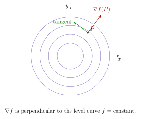
Proposition 3.40 (Gradient and level sets). If $F:\mathbb{R}^n\to\mathbb{R}$ is differentiable and $F(\boldsymbol{x})=c$ defines a level set, then $\nabla F(\boldsymbol{x})$ is orthogonal to the level set at points where $\nabla F(\boldsymbol{x})\neq \boldsymbol{0}$.

Remark 118 (Geometric meaning). Level curves/surfaces are “stay at the same height.” The gradient points in the direction that changes the height most, so it must be perpendicular to “no change” directions.

Exercise 3.42. Let $F(x,y,z)=x e^{yz}+z-2=0$ define $z=z(x,y)$ near a point where $F_z\neq 0$. Compute $z_x$ and $z_y$ using Theorem 3.38.

Chapter 3 Checklist

Interpret $z=f(x,y)$ as a surface; use slices and level curves to visualize it (Lesson 3.1).
Use the $\varepsilon$–$\delta$ definition of limit in $\mathbb{R}^2$ and the path test to disprove limits (Lesson 3.2).
Compute partial derivatives and mixed partials; apply Clairaut under continuity (Lesson 3.3).
Understand differentiability as “best linear approximation” Definition 3.23; use $\nabla f$ and directional derivatives Theorem 3.30 (Lesson 3.4).
Apply the multivariable chain rule Theorems 3.34 and 3.37 and implicit differentiation Theorem 3.38 (Lesson 3.5).

4 Chapter 4: Applications of Partial Derivatives

Key Idea

Partial derivatives are not just computational objects. They encode local geometry (tangent planes and best linear approximations) and local shape (max/min/saddle behavior). Chapter 4 is the “toolbox chapter”: once you can linearize and optimize reliably, many applied problems (physics, economics, data fitting) become routine.

4.1 Lesson 4.1: Tangent Planes and Linear Approximations

4.1.1 Tangent Plane to a Surface $z=f(x,y)$

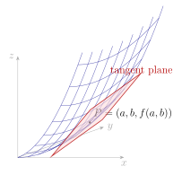
Theorem 4.1 (Tangent plane equation). Let $f$ be differentiable at $(a,b)$, and consider the surface $z=f(x,y)$. The tangent plane at the point $(a,b,f(a,b))$ is \[\begin{equation} z = f(a,b) + f_x(a,b)(x-a) + f_y(a,b)(y-b). \end{equation}\]

Remark 121 (Why this is the right formula). Differentiability means: near $(a,b)$, $f$ is well-approximated by a linear map in $(x-a,y-b)$. A plane is exactly “constant + linear terms,” so Theorem 4.1 is the geometric translation of “best linear approximation.”

Example 4.3 (Compute a tangent plane). Let $f(x,y)=x^2+2y^2$ and take $(a,b)=(1,-1)$. Then \[f(1,-1)=1+2=3,\qquad f_x(x,y)=2x,\qquad f_y(x,y)=4y.\] So $f_x(1,-1)=2$ and $f_y(1,-1)=-4$. The tangent plane is \[z = 3 + 2(x-1) - 4(y+1) \quad\Longleftrightarrow\quad z = 2x - 4y - 3.\]

A surface patch and its tangent plane at a point: the plane is the best local linear fit.

4.1.2 Linearization (Best Local Linear Approximation)

Definition 4.4 (Linearization). If $f$ is differentiable at $(a,b)$, its linearization at $(a,b)$ is the linear function \[\begin{equation} L(x,y)= f(a,b) + f_x(a,b)(x-a) + f_y(a,b)(y-b). \end{equation}\] Then $f(x,y)\approx L(x,y)$ for $(x,y)$ near $(a,b)$.

Remark 124 (What you should remember). Linearization is “tangent plane as a formula.” When you need a quick approximation, compute $f(a,b)$ and the two partial derivatives there, and plug into Definition 4.4.

Example 4.6 (Fast approximation with small changes). Approximate $\sqrt{(4.02)^2 + (0.01)^2}$ without a calculator.

Let $f(x,y)=\sqrt{x^2+y^2}$ and expand near $(a,b)=(4,0)$. Compute: \[f(4,0)=4,\qquad f_x(x,y)=\frac{x}{\sqrt{x^2+y^2}},\qquad f_y(x,y)=\frac{y}{\sqrt{x^2+y^2}}.\] So $f_x(4,0)=1$ and $f_y(4,0)=0$. Then \[L(x,y)=4+1(x-4)+0(y-0)=x.\] Now take $(x,y)=(4.02,0.01)$: \[f(4.02,0.01)\approx L(4.02,0.01)=4.02.\] (The $y$-change contributes only at second order because $f_y(4,0)=0$.)

4.1.3 Error Estimates (Second-Order Control)

Theorem 4.7 (Second-order Taylor form with remainder). Assume $f$ has continuous second partial derivatives on a neighborhood of $(a,b)$. For $(x,y)=(a+h,b+k)$ near $(a,b)$, there exist points along the line segment from $(a,b)$ to $(a+h,b+k)$ such that \[\begin{equation} f(a+h,b+k)=f(a,b)+f_x(a,b)h+f_y(a,b)k+\frac12\Big(f_{xx}(\xi,\eta)h^2+2f_{xy}(\xi,\eta)hk+f_{yy}(\xi,\eta)k^2\Big). \end{equation}\]

Corollary 4.8 (A usable error bound for linearization). Suppose $|f_{xx}|,|f_{xy}|,|f_{yy}| \le M$ on a neighborhood containing the segment from $(a,b)$ to $(x,y)=(a+h,b+k)$. Then the linearization error satisfies \[\begin{equation} |f(a+h,b+k)-L(a+h,b+k)| \le \frac{M}{2}\big(|h|+|k|\big)^2 \le M(h^2+k^2). \end{equation}\]

Proof. From Theorem 4.7, the error equals the absolute value of the second-order term: \[\begin{align*} \left|\frac12\big(f_{xx}h^2+2f_{xy}hk+f_{yy}k^2\big)\right| &\le \frac12\Big(|f_{xx}|\,h^2+2|f_{xy}|\,|hk|+|f_{yy}|\,k^2\Big) \\ &\le \frac{M}{2}\big(h^2+2|hk|+k^2\big) \\ &= \frac{M}{2}(|h|+|k|)^2. \end{align*}\] Also $(|h|+|k|)^2 \le 2(h^2+k^2)$, hence the weaker bound $\le M(h^2+k^2)$. ◻

Exercise 4.9. Let $f(x,y)=e^{x+y}$. Linearize at $(0,0)$ and approximate $e^{0.02-0.01}$. Then use Corollary 4.8 with a reasonable bound $M$ on second partial derivatives near $(0,0)$ to estimate the error.

4.2 Lesson 4.2: Extrema of Functions of Several Variables

4.2.1 Critical Points and Local Extrema

Definition 4.10 (Local maximum/minimum). Let $f:D\subset\mathbb{R}^2\to\mathbb{R}$ and $(a,b)\in D$.

$f$ has a local maximum at $(a,b)$ if $f(a,b)\ge f(x,y)$ for all $(x,y)$ in some neighborhood of $(a,b)$ within $D$.
$f$ has a local minimum at $(a,b)$ if $f(a,b)\le f(x,y)$ for all $(x,y)$ in some neighborhood of $(a,b)$ within $D$.

Definition 4.11 (Critical point). Assume $f_x$ and $f_y$ exist. An interior point $(a,b)$ is a critical point if \[f_x(a,b)=0 \quad \text{and}\quad f_y(a,b)=0,\] or if at least one of $f_x(a,b),f_y(a,b)$ does not exist.

Theorem 4.12 (Fermat’s theorem in two variables). If $f$ has a local max or local min at an interior point $(a,b)$ and $f_x,f_y$ exist at $(a,b)$, then \[f_x(a,b)=0,\qquad f_y(a,b)=0.\]

Remark 132 (Common pitfall). Theorem 4.12 is one-way: critical points are candidates for extrema, not guaranteed extrema. You must still classify them (Lesson 4.3) or check boundaries for global problems.

4.2.2 Global Extrema on Closed and Bounded Regions

Theorem 4.14 (Extreme Value Theorem (EVT) in $\mathbb{R}^2$). If $f$ is continuous on a closed and bounded set $D\subset\mathbb{R}^2$, then $f$ attains both an absolute maximum and an absolute minimum on $D$.

Proposition 4.15 (Practical recipe for global extrema). To find absolute extrema of continuous $f$ on a closed, bounded region $D$:

Find all critical points in the interior of $D$ and evaluate $f$ there.
Analyze the boundary $\partial D$ (often by parameterizing it or reducing to a single-variable problem) and evaluate $f$ on boundary critical points/endpoints.
Compare all values; the largest is the absolute max and the smallest is the absolute min.

Example 4.16 (Absolute extrema on a disk). Find the absolute max/min of $f(x,y)=x^2+y^2-2x$ on the closed disk $D=\{(x,y):x^2+y^2\le 4\}$.

Step 1 (interior critical points). \[f_x=2x-2,\qquad f_y=2y.\] Set $f_x=f_y=0$ gives $(x,y)=(1,0)$, which lies in $D$. Then $f(1,0)=1-2=-1$.

Step 2 (boundary). On $\partial D$, $x^2+y^2=4$. Then \[f=x^2+y^2-2x=4-2x.\] So maximizing/minimizing $f$ on the boundary is the same as minimizing/maximizing $x$ on the circle. On $x^2+y^2=4$, we have $-2\le x\le 2$. Thus \[f_{\min,\partial D}=4-2(2)=0 \quad \text{at }(2,0), \qquad f_{\max,\partial D}=4-2(-2)=8 \quad \text{at }(-2,0).\]

Step 3 (compare). Candidate values: $-1$ (interior), $0$ and $8$ (boundary). So the absolute minimum is $-1$ at $(1,0)$ and the absolute maximum is $8$ at $(-2,0)$.

Exercise 4.17. Find the absolute max and min of $f(x,y)=xy$ on the triangle with vertices $(0,0)$, $(2,0)$, $(0,3)$. (Hint: boundary consists of three line segments; reduce each to a single-variable function.)

4.3 Lesson 4.3: The Second Derivative Test

4.3.1 The Hessian Matrix and Quadratic Approximation

Definition 4.18 (Hessian in $\mathbb{R}^2$). If $f$ has second partial derivatives, the Hessian matrix is \[H_f(x,y)= \begin{pmatrix} f_{xx}(x,y) & f_{xy}(x,y)\\ f_{yx}(x,y) & f_{yy}(x,y) \end{pmatrix}.\] If the mixed partials are continuous, then $f_{xy}=f_{yx}$ by Clairaut’s theorem, so $H_f$ is symmetric.

Remark 138 (Why the Hessian matters). Near a critical point, the first-order (linear) part is zero, so the second-order terms dominate. The Hessian tells you whether the surface bends upward (minimum), downward (maximum), or in opposite directions (saddle).

4.3.2 Classification in Two Variables

Theorem 4.20 (Second derivative test in $\mathbb{R}^2$). Let $f$ have continuous second partial derivatives near $(a,b)$, and suppose $(a,b)$ is a critical point with $f_x(a,b)=f_y(a,b)=0$. Define \[\begin{equation} D = f_{xx}(a,b)\,f_{yy}(a,b) - \big(f_{xy}(a,b)\big)^2. \end{equation}\] Then:

If $D>0$ and $f_{xx}(a,b)>0$, then $f$ has a local minimum at $(a,b)$.
If $D>0$ and $f_{xx}(a,b)<0$, then $f$ has a local maximum at $(a,b)$.
If $D<0$, then $(a,b)$ is a saddle point (neither max nor min).
If $D=0$, the test is inconclusive.

Remark 140 (In plain language). $D$ measures whether the quadratic form bends the same way in all directions.

$D>0$ means the quadratic part is definite (up or down), so you get a min or max.
$D<0$ means it bends up in some directions and down in others: saddle.

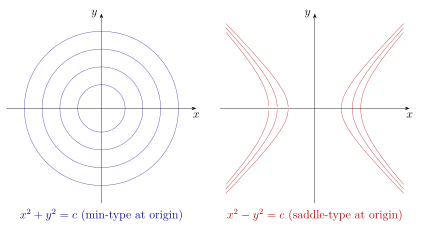
Example 4.22 (One min, one saddle, one max).

$f(x,y)=x^2+y^2$. Critical point at $(0,0)$. Here $f_{xx}=2$, $f_{yy}=2$, $f_{xy}=0$, so $D=4>0$ and $f_{xx}>0$. Local minimum.
$g(x,y)=x^2-y^2$. Critical point at $(0,0)$. Here $g_{xx}=2$, $g_{yy}=-2$, $g_{xy}=0$, so $D=-4<0$. Saddle point.
$h(x,y)=-(x^2+y^2)$. Critical point at $(0,0)$. Here $h_{xx}=-2$, $h_{yy}=-2$, $h_{xy}=0$, so $D=4>0$ and $h_{xx}<0$. Local maximum.

Contour patterns distinguish local minima (nested ovals) from saddles (hyperbolic contours).

Exercise 4.23. Classify all critical points of $f(x,y)=x^3-3x+y^2$ using Theorem 4.20. (Compute $f_x,f_y$, solve for critical points, then compute $D$.)

4.4 Lesson 4.4: Constrained Optimization

4.4.1 Lagrange Multipliers: Statement

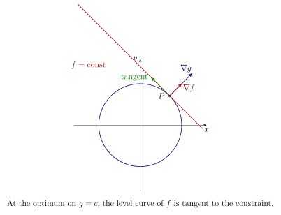
Theorem 4.24 (Lagrange multipliers (one constraint)). Let $f,g:\mathbb{R}^2\to\mathbb{R}$ have continuous partial derivatives. Suppose $f$ has a local maximum or minimum on the constraint curve \[g(x,y)=c\] at a point $(a,b)$ where $\nabla g(a,b)\neq \boldsymbol{0}$. Then there exists a scalar $\lambda$ such that \[\begin{equation} \nabla f(a,b)=\lambda\,\nabla g(a,b). \end{equation}\]

Remark 144 (Geometric meaning (the one picture to remember)). Along the constraint $g=c$, you are allowed to move only tangent to the curve. At an extremum, moving tangent should not change $f$ (no first-order increase/decrease). That means $\nabla f$ must be perpendicular to the tangent direction. But $\nabla g$ is also perpendicular to the constraint curve (it is normal to $g=c$). So the two normals are parallel: $\nabla f=\lambda \nabla g$.

Lagrange multipliers: at a constrained extremum, $\nabla f$ and $\nabla g$ are parallel.

4.4.2 How to Use Lagrange Multipliers (Algorithm)

Proposition 4.26 (Computational procedure). To optimize $f(x,y)$ subject to $g(x,y)=c$:

Compute gradients $\nabla f=\langle f_x,f_y\rangle$ and $\nabla g=\langle g_x,g_y\rangle$.
Solve the system \[\nabla f(x,y)=\lambda \nabla g(x,y),\qquad g(x,y)=c\] for $(x,y,\lambda)$.
Evaluate $f$ at the candidate points and decide which are max/min (often by comparison, or using context).

4.4.3 Worked Examples

Example 4.27 (Max/min of a product on a circle). Find the maximum and minimum of $f(x,y)=xy$ subject to $g(x,y)=x^2+y^2=1$.

Compute gradients: \[\nabla f=\langle y,\ x\rangle,\qquad \nabla g=\langle 2x,\ 2y\rangle.\] Set $\nabla f=\lambda \nabla g$: \[y=2\lambda x,\qquad x=2\lambda y,\qquad x^2+y^2=1.\] If $x=0$, then $y^2=1$ so $y=\pm 1$, and $f=0$. If $x\neq 0$ and $y\neq 0$, substitute $y=2\lambda x$ into $x=2\lambda y$: \[x=2\lambda(2\lambda x)=4\lambda^2 x \quad\Rightarrow\quad 4\lambda^2=1 \Rightarrow \lambda=\pm\frac12.\] If $\lambda=\tfrac12$, then $y=x$ and $x^2+y^2=2x^2=1$, so $x=\pm\frac{1}{\sqrt2}$ and $y=\pm\frac{1}{\sqrt2}$ (same sign). Then $f=xy=\frac12$. If $\lambda=-\tfrac12$, then $y=-x$ and $2x^2=1$, so $x=\pm\frac{1}{\sqrt2}$ and $y=\mp\frac{1}{\sqrt2}$ (opposite signs). Then $f=-\frac12$.

So the maximum is $\frac12$ at $\left(\frac{1}{\sqrt2},\frac{1}{\sqrt2}\right)$ and $\left(-\frac{1}{\sqrt2},-\frac{1}{\sqrt2}\right)$, and the minimum is $-\frac12$ at $\left(\frac{1}{\sqrt2},-\frac{1}{\sqrt2}\right)$ and $\left(-\frac{1}{\sqrt2},\frac{1}{\sqrt2}\right)$.

Example 4.28 (Distance to a line: closest point). Find the point on the line $x+y=1$ closest to the origin.

Minimize squared distance $f(x,y)=x^2+y^2$ subject to $g(x,y)=x+y=1$. \[\nabla f=\langle 2x,2y\rangle,\qquad \nabla g=\langle 1,1\rangle.\] Set $\nabla f=\lambda \nabla g$: \[2x=\lambda,\qquad 2y=\lambda,\qquad x+y=1.\] Thus $x=y$, so $2x=1$ and $x=y=\frac12$. The closest point is $\left(\frac12,\frac12\right)$, and the minimum distance is $\sqrt{\left(\frac12\right)^2+\left(\frac12\right)^2}=\frac{1}{\sqrt2}$.

Exercise 4.29. Use Lagrange multipliers to find the maximum and minimum of $f(x,y)=x^2+2y^2$ subject to $x^2+y^2=3$. (Your final answers should be specific points and corresponding max/min values.)

Chapter 4 Checklist

Tangent plane / linearization at $(a,b)$: \[L(x,y)=f(a,b)+f_x(a,b)(x-a)+f_y(a,b)(y-b).\]
Use second derivatives to control approximation error (Taylor + bounds) Corollary 4.8.
Local extrema candidates: interior critical points Definition 4.11; global extrema on closed bounded sets via EVT Theorem 4.14.
Classify critical points using the second derivative test Theorem 4.20.
Constrained optimization: solve $\nabla f=\lambda \nabla g$ plus the constraint equation Theorem 4.24.

5 Chapter 5: Multiple Integrals

Key Idea

Single-variable integration adds up tiny line segments. Double integrals add up tiny area elements $dA$ over a region in the plane. Triple integrals add up tiny volume elements $dV$ over a region in space.

The most intuitive understanding: divide a region into many very small pieces (small rectangles/small boxes), on each small piece compute "function value $\times$ area/volume of small piece", then add them all up—the limit is the multiple integral.

5.1 Lesson 5.1: Double Integrals over Rectangular Regions

5.1.1 Definition of Double Integrals

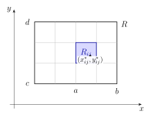
Definition 5.1 (Double integral over a rectangle). Let $R=[a,b]\times[c,d]\subset\mathbb{R}^2$ and let $f$ be bounded on $R$. Partition $[a,b]$ into $m$ subintervals and $[c,d]$ into $n$ subintervals, forming subrectangles \[R_{ij}=[x_{i-1},x_i]\times[y_{j-1},y_j],\qquad \Delta A_{ij}=(x_i-x_{i-1})(y_j-y_{j-1}).\] Choose a sample point $(x_{ij}^*,y_{ij}^*)\in R_{ij}$ and form the Riemann sum \[S=\sum_{i=1}^{m}\sum_{j=1}^{n} f(x_{ij}^*,y_{ij}^*)\,\Delta A_{ij}.\] If $S$ approaches a limit as $\max\{\Delta x_i,\Delta y_j\}\to 0$ (independent of sample points), then $f$ is integrable on $R$ and we define \[\iint_R f(x,y)\,dA=\lim_{\max\{\Delta x_i,\Delta y_j\}\to 0}\sum_{i=1}^{m}\sum_{j=1}^{n} f(x_{ij}^*,y_{ij}^*)\,\Delta A_{ij}.\]

Remark 150 (A safe existence condition). If $f$ is continuous on the rectangle $R$, then $f$ is integrable on $R$ and the double integral exists.

A rectangle region partitioned into small subrectangles $R_{ij}$; the double integral is the limit of sums $f(x^*_{ij},y^*_{ij})\Delta A_{ij}$.

5.1.2 Iterated Integrals

Theorem 5.3 (Iterated integral over a rectangle). If $f$ is continuous on $R=[a,b]\times[c,d]$, then \[\begin{equation} \iint_R f(x,y)\,dA=\int_{a}^{b}\left(\int_{c}^{d} f(x,y)\,dy\right)\,dx =\int_{c}^{d}\left(\int_{a}^{b} f(x,y)\,dx\right)\,dy. \end{equation}\]

Remark 152 (Intuitive understanding). In a rectangular region, you can first "add up each vertical strip in the $y$ direction" (inner integral), then sum all the vertical strips over $x$ (outer integral). You can also reverse the order: first along $x$ then along $y$. The advantage of rectangles is that the upper, lower, left, and right boundaries are all constants.

Example 5.5 (Compute a double integral on a rectangle). Let $R=[0,1]\times[0,2]$ and $f(x,y)=x+y$. Then \[\iint_R (x+y)\,dA=\int_{0}^{1}\int_{0}^{2}(x+y)\,dy\,dx.\] Compute the inner integral: \[\int_{0}^{2}(x+y)\,dy=\Big(xy+\tfrac12 y^2\Big)\Big|_{0}^{2}=2x+2.\] Then \[\int_{0}^{1}(2x+2)\,dx=\big(x^2+2x\big)\Big|_{0}^{1}=1+2=3.\] So $\iint_R (x+y)\,dA=3$.

5.1.3 Fubini’s Theorem

Theorem 5.6 (Fubini’s Theorem (practical version)). If $f$ is continuous on a rectangle $R$, then both iterated integrals in Theorem 5.3 exist and are equal to $\iint_R f\,dA$. More generally, if $\iint_R |f|\,dA<\infty$ (absolute integrability), then the iterated integrals exist and are equal.

Exercise 5.7. Compute $\iint_{[1,3]\times[0,1]} (2x-3y)\,dA$ in two ways: \[\int_{1}^{3}\int_{0}^{1}(2x-3y)\,dy\,dx \quad\text{and}\quad \int_{0}^{1}\int_{1}^{3}(2x-3y)\,dx\,dy.\] Verify the answers match.

5.2 Lesson 5.2: Double Integrals over General Regions

5.2.1 Type I and Type II Regions

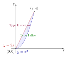
Definition 5.8 (Type I (vertically simple) region). A region $D\subset\mathbb{R}^2$ is Type I if it can be described as \[D=\{(x,y): a\le x\le b,\ g_1(x)\le y\le g_2(x)\},\] for some functions $g_1,g_2$ with $g_1(x)\le g_2(x)$ on $[a,b]$.

Definition 5.9 (Type II (horizontally simple) region). A region $D\subset\mathbb{R}^2$ is Type II if it can be described as \[D=\{(x,y): c\le y\le d,\ h_1(y)\le x\le h_2(y)\},\] for some functions $h_1,h_2$ with $h_1(y)\le h_2(y)$ on $[c,d]$.

Theorem 5.10 (Integrating over Type I / Type II regions). If $f$ is continuous on $D$, then \[\iint_D f(x,y)\,dA=\int_{a}^{b}\int_{g_1(x)}^{g_2(x)} f(x,y)\,dy\,dx \quad (\text{Type I}),\] \[\iint_D f(x,y)\,dA=\int_{c}^{d}\int_{h_1(y)}^{h_2(y)} f(x,y)\,dx\,dy \quad (\text{Type II}).\]

Remark 159 (Intuitive understanding). Type I: use "vertical slices," fix $x$, $y$ goes from lower boundary $g_1(x)$ to upper boundary $g_2(x)$. Type II: use "horizontal slices," fix $y$, $x$ goes from left boundary $h_1(y)$ to right boundary $h_2(y)$. The same region can often be represented using either Type I or Type II; choose whichever is simpler.

A region that is both Type I and Type II: between $y=x^2$ and $y=2x$ in the first quadrant.

5.2.2 Changing the Order of Integration

Proposition 5.12 (How to change the order (workflow)). Given an iterated integral, to switch $dy\,dx$ to $dx\,dy$ (or vice versa):

Sketch the region $D$ described by the current bounds.
Decide whether you want vertical slices (Type I) or horizontal slices (Type II).
Rewrite $D$ with the new slice description (new outer bounds + new inner bounds).
Rewrite the integral with the new bounds; then integrate.

Example 5.13 (Change order for the region between $y=x^2$ and $y=2x$). Let $D=\{(x,y):0\le x\le 2,\ x^2\le y\le 2x\}$. Then \[\iint_D 1\,dA=\int_{0}^{2}\int_{x^2}^{2x} 1\,dy\,dx.\] Compute directly: \[\int_{0}^{2}\big(2x-x^2\big)\,dx=\Big(x^2-\tfrac13 x^3\Big)\Big|_{0}^{2}=4-\tfrac83=\tfrac{4}{3}.\]

Now rewrite as Type II. Here $y$ ranges from $0$ to $4$. For a fixed $y\in[0,4]$, $x$ runs from the line $y=2x$ (i.e. $x=y/2$) to the parabola $y=x^2$ (i.e. $x=\sqrt{y}$): \[D=\{(x,y):0\le y\le 4,\ \tfrac{y}{2}\le x\le \sqrt{y}\}.\] Thus \[\iint_D 1\,dA=\int_{0}^{4}\int_{y/2}^{\sqrt{y}} 1\,dx\,dy =\int_{0}^{4}\left(\sqrt{y}-\frac{y}{2}\right)\,dy =\left(\frac{2}{3}y^{3/2}-\frac14 y^2\right)\Big|_{0}^{4} =\frac{16}{3}-4=\frac{4}{3},\] which matches, as it must.

Exercise 5.14. Rewrite and evaluate \[\int_{0}^{1}\int_{x}^{1} e^{y^2}\,dy\,dx\] by switching the order of integration. (Hint: the integrand suggests $dx$ inside.)

5.3 Lesson 5.3: Applications of Double Integrals

5.3.1 Area and Volume

Proposition 5.15 (Area of a planar region). If $D\subset\mathbb{R}^2$ is a region with finite area, then \[\operatorname{Area}(D)=\iint_D 1\,dA.\]

Proposition 5.16 (Volume under a surface). If $f(x,y)\ge 0$ on $D$, then the volume under $z=f(x,y)$ above $D$ is \[V=\iint_D f(x,y)\,dA.\] If $f$ changes sign, $\iint_D f\,dA$ is a signed volume; geometric volume is typically $\iint_D |f|\,dA$.

Remark 165 (Intuitive understanding). $\iint_D 1\,dA$ is "counting each small area element once," so it yields the total area. $\iint_D f\,dA$ is multiplying the "height $f$" of each small piece by its "base area $dA$," and adding them up gives the volume (when $f\ge0$).

5.3.2 Mass and Density

Proposition 5.18 (Mass of a lamina). If a thin plate occupies region $D$ with (possibly varying) surface density $\rho(x,y)\ge 0$ (mass per unit area), then its mass is \[m=\iint_D \rho(x,y)\,dA.\]

5.3.3 Average Value

Definition 5.19 (Average value on a region). If $f$ is integrable on $D$ and $\operatorname{Area}(D)>0$, the average value of $f$ on $D$ is \[f_{\text{avg}}=\frac{1}{\operatorname{Area}(D)}\iint_D f(x,y)\,dA.\]

Example 5.20 (Mass with variable density on a triangular region). Let $D=\{(x,y): 0\le x\le 1,\ 0\le y\le 2x\}$ (a triangle). Let density be $\rho(x,y)=x+y$. Then \[m=\iint_D (x+y)\,dA=\int_{0}^{1}\int_{0}^{2x} (x+y)\,dy\,dx.\] Compute the inner integral: \[\int_{0}^{2x}(x+y)\,dy=\Big(xy+\tfrac12 y^2\Big)\Big|_{0}^{2x}=2x^2+2x^2=4x^2.\] Then \[m=\int_{0}^{1}4x^2\,dx=\frac{4}{3}.\] Also $\operatorname{Area}(D)=\int_{0}^{1}\int_{0}^{2x}1\,dy\,dx=\int_{0}^{1}2x\,dx=1$. So the average density (and the average of $x+y$ over $D$) is $m/\operatorname{Area}(D)=\frac{4}{3}$.

Example 5.21 (Average value over a rectangle). Let $R=[0,2]\times[0,1]$ and $f(x,y)=x^2+2y$. \[\begin{align*} \iint_R f\,dA &= \int_{0}^{2}\int_{0}^{1}(x^2+2y)\,dy\,dx = \int_{0}^{2}\Big(x^2y+y^2\Big)\Big|_{0}^{1}\,dx \\ &= \int_{0}^{2}(x^2+1)\,dx = \Big(\tfrac13 x^3+x\Big)\Big|_{0}^{2} = \frac{8}{3}+2=\frac{14}{3}. \end{align*}\] Area$(R)=2$. Hence \[f_{\text{avg}}=\frac{1}{2}\cdot\frac{14}{3}=\frac{7}{3}.\]

Exercise 5.22. Find the volume under $z=3-x-y$ above the triangle with vertices $(0,0)$, $(3,0)$, $(0,2)$. (First confirm $3-x-y\ge0$ on the region.)

5.4 Lesson 5.4: Polar Coordinates

5.4.1 Polar Coordinate System

Definition 5.23 (Polar coordinates). Polar coordinates represent a point in the plane by $(r,\theta)$ where \[x=r\cos\theta,\qquad y=r\sin\theta,\qquad r\ge 0.\] Also \[r=\sqrt{x^2+y^2},\qquad \theta=\text{angle from the positive $x$-axis (chosen consistently).}\]

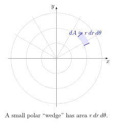
Proposition 5.24 (Area element in polar coordinates). Under the change of variables $(x,y)=(r\cos\theta,r\sin\theta)$, the area element transforms as \[\begin{equation} dA = r\,dr\,d\theta. \end{equation}\]

Remark 173 (Intuitive understanding). At a fixed angle $\theta$, as the radius increases from $r$ to $r+dr$, it forms a "thin annular wedge" with area approximately \[(\text{arc length})\times(\text{thickness}) \approx (r\,d\theta)\cdot(dr)=r\,dr\,d\theta,\] which is the extra factor of $r$ in Proposition 5.24.

Polar coordinates: the Jacobian factor $r$ comes from the arc length $r\,d\theta$.

5.4.2 Double Integrals in Polar Coordinates

Theorem 5.26 (Polar-coordinate double integral). Let $D$ be described in polar form by \[\alpha\le \theta\le \beta,\qquad 0\le r\le g(\theta),\] and let $f$ be integrable on $D$. Then \[\begin{equation} \iint_D f(x,y)\,dA = \int_{\alpha}^{\beta}\int_{0}^{g(\theta)} f(r\cos\theta,r\sin\theta)\, r\,dr\,d\theta. \end{equation}\] More generally, if $r$ ranges between two curves $r=g_1(\theta)$ and $r=g_2(\theta)$, then use $g_1(\theta)\le r\le g_2(\theta)$.

5.4.3 Applications

Example 5.27 (Area of a disk). For the disk $x^2+y^2\le a^2$, we have $0\le r\le a$ and $0\le\theta\le 2\pi$. Then \[\operatorname{Area}=\iint_D 1\,dA =\int_{0}^{2\pi}\int_{0}^{a} 1\cdot r\,dr\,d\theta =\int_{0}^{2\pi}\left(\tfrac12 a^2\right)d\theta =\pi a^2.\]

Example 5.28 (A common integrand: $x^2+y^2$ over a disk). Let $D=\{(x,y):x^2+y^2\le a^2\}$ and $f(x,y)=x^2+y^2$. In polar, $f=r^2$. Thus \[\iint_D (x^2+y^2)\,dA =\int_{0}^{2\pi}\int_{0}^{a} r^2\cdot r\,dr\,d\theta =\int_{0}^{2\pi}\int_{0}^{a} r^3\,dr\,d\theta =\int_{0}^{2\pi}\left(\tfrac14 a^4\right)d\theta =\frac{\pi}{2}a^4.\]

Exercise 5.29. Evaluate $\iint_D \sqrt{x^2+y^2}\,dA$ over the annulus $1\le x^2+y^2\le 4$ using polar coordinates.

5.5 Lesson 5.5: Triple Integrals

5.5.1 Definition of Triple Integrals

Definition 5.30 (Triple integral over a box). Let $B=[a,b]\times[c,d]\times[e,f]\subset\mathbb{R}^3$, and let $F$ be bounded on $B$. Partition $B$ into small boxes $B_{ijk}$ with volume $\Delta V_{ijk}$ and choose sample points $(x_{ijk}^*,y_{ijk}^*,z_{ijk}^*)$. If the Riemann sums \[\sum_{i}\sum_{j}\sum_{k} F(x_{ijk}^*,y_{ijk}^*,z_{ijk}^*)\,\Delta V_{ijk}\] approach a limit as the mesh goes to $0$, we define \[\iiint_B F(x,y,z)\,dV=\lim \sum_{i}\sum_{j}\sum_{k} F(x_{ijk}^*,y_{ijk}^*,z_{ijk}^*)\,\Delta V_{ijk}.\]

Remark 179 (Intuitive understanding). Divide the spatial region into many small boxes, each small box contributes approximately $F\cdot(\text{volume of small box})$, add them all up and take the limit to get the triple integral.

5.5.2 Triple Integrals in Rectangular Coordinates (Fubini)

Theorem 5.32 (Iterated integrals for a box). If $F$ is continuous on the box $B=[a,b]\times[c,d]\times[e,f]$, then \[\iiint_B F(x,y,z)\,dV = \int_{a}^{b}\int_{c}^{d}\int_{e}^{f} F(x,y,z)\,dz\,dy\,dx,\] and similarly for the other 5 possible integration orders.

5.5.3 Applications to Volume and Mass

Proposition 5.33 (Volume of a solid). If $E\subset\mathbb{R}^3$ is a solid region with finite volume, then \[\operatorname{Vol}(E)=\iiint_E 1\,dV.\]

Proposition 5.34 (Mass of a solid). If a solid occupies $E$ with density $\rho(x,y,z)\ge 0$ (mass per unit volume), then \[m=\iiint_E \rho(x,y,z)\,dV.\]

Definition 5.35 (Average value in 3D). If $F$ is integrable on $E$ and $\operatorname{Vol}(E)>0$, then \[F_{\text{avg}}=\frac{1}{\operatorname{Vol}(E)}\iiint_E F\,dV.\]

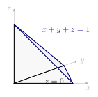
Example 5.36 (Volume of the tetrahedron $x+y+z\le 1$ in the first octant). Let \[E=\{(x,y,z): x\ge 0,\ y\ge 0,\ z\ge 0,\ x+y+z\le 1\}.\] A convenient description is \[0\le x\le 1,\qquad 0\le y\le 1-x,\qquad 0\le z\le 1-x-y.\] Thus \[\operatorname{Vol}(E)=\iiint_E 1\,dV =\int_{0}^{1}\int_{0}^{1-x}\int_{0}^{1-x-y} 1\,dz\,dy\,dx.\] Integrate: \[\int_{0}^{1-x-y}1\,dz=1-x-y,\] \[\int_{0}^{1-x}(1-x-y)\,dy=\Big((1-x)y-\tfrac12 y^2\Big)\Big|_{0}^{1-x} =\frac{(1-x)^2}{2},\] \[\int_{0}^{1}\frac{(1-x)^2}{2}\,dx =\frac12\int_{0}^{1}(1-2x+x^2)\,dx =\frac12\Big(x-x^2+\tfrac13 x^3\Big)\Big|_{0}^{1} =\frac12\cdot\frac13=\frac{1}{6}.\] So $\operatorname{Vol}(E)=\frac{1}{6}$.

Example 5.37 (Mass with density $\rho=z$ on the same tetrahedron). Using the same region $E$ as Example 5.36 with density $\rho(x,y,z)=z$, \[m=\iiint_E z\,dV =\int_{0}^{1}\int_{0}^{1-x}\int_{0}^{1-x-y} z\,dz\,dy\,dx.\] Compute: \[\int_{0}^{1-x-y} z\,dz=\frac{(1-x-y)^2}{2}.\] Then \[\int_{0}^{1-x}\frac{(1-x-y)^2}{2}\,dy =\frac12\int_{0}^{1-x} (1-x-y)^2\,dy.\] Let $u=1-x-y$ so $du=-dy$, and when $y=0$, $u=1-x$, when $y=1-x$, $u=0$: \[\frac12\int_{u=1-x}^{0} u^2(-du)=\frac12\int_{0}^{1-x}u^2\,du=\frac12\cdot\frac{(1-x)^3}{3}=\frac{(1-x)^3}{6}.\] Finally \[m=\int_{0}^{1}\frac{(1-x)^3}{6}\,dx =\frac{1}{6}\int_{0}^{1}(1-3x+3x^2-x^3)\,dx =\frac{1}{6}\left(1-\frac{3}{2}+1-\frac{1}{4}\right) =\frac{1}{6}\cdot\frac{1}{4} =\frac{1}{24}.\] So $m=\frac{1}{24}$, and the average value of $z$ over $E$ is \[z_{\text{avg}}=\frac{m}{\operatorname{Vol}(E)}=\frac{1/24}{1/6}=\frac{1}{4}.\]

The solid $x,y,z\ge 0$ and $x+y+z\le 1$ (a tetrahedron). Triple integrals add up $F\,dV$ over such a region.

Exercise 5.38. Set up (do not necessarily evaluate) an iterated integral for $\iiint_E (x+2y+3z)\,dV$ where $E$ is bounded by \[0\le z\le 2,\qquad 0\le y\le 1,\qquad 0\le x\le 3-y.\] Then compute the volume of $E$ using $\iiint_E 1\,dV$.

Chapter 5 Checklist

Double integral definition: limit of sums $f(x^*,y^*)\Delta A$ over partitions (Lesson 5.1).
Rectangle $\Rightarrow$ iterated integrals and order swap via Fubini (Theorem Theorem 5.6).
General regions: Type I (vertical slices) and Type II (horizontal slices) (Lesson 5.2).
Changing order: sketch $D$, rewrite bounds, then integrate (Proposition Proposition 5.12).
Applications: area $\iint_D 1\,dA$, volume $\iint_D f\,dA$ (for $f\ge0$), mass $\iint_D \rho\,dA$, average value (Lesson 5.3).
Polar coordinates: $(x,y)=(r\cos\theta,r\sin\theta)$ and $dA=r\,dr\,d\theta$ (Lesson 5.4).
Triple integrals: $\iiint_E F\,dV$; volume $\iiint_E 1\,dV$; mass $\iiint_E \rho\,dV$ (Lesson 5.5).

6 Chapter 6: Change of Variables in Multiple Integrals

Key Idea

A change of variables is the multivariable analogue of substitution in single-variable calculus.

If a mapping $(u,v)\mapsto (x,y)$ is smooth and one-to-one, then small area elements scale by a factor \[\left|\frac{\partial(x,y)}{\partial(u,v)}\right|\] (the Jacobian). This turns complicated regions in the $xy$-plane into simpler regions in the $uv$-plane, where integrals are easier to set up and compute.

6.1 Lesson 6.1: Jacobians and Coordinate Transformations

6.1.1 Motivation for Change of Variables

Remark 187 (Why we bother). The hard part of many double/triple integrals is not the integrand; it is the region. A well-chosen coordinate transformation can turn “curved boundaries” into “constant bounds,” while the Jacobian keeps the calculation honest by correcting the area/volume scale.

6.1.2 Transformations and the Jacobian Determinant

Definition 6.2 (Planar transformation). A (planar) coordinate transformation is a mapping \[T:\ (u,v)\mapsto (x,y)=(x(u,v),y(u,v)),\] defined on a region $D^\ast$ in the $uv$-plane and mapping it to a region $D=T(D^\ast)$ in the $xy$-plane.

Definition 6.3 (Jacobian determinant). Assume $x(u,v)$ and $y(u,v)$ have continuous first partial derivatives. The Jacobian determinant of $T$ is \[\begin{equation} \frac{\partial(x,y)}{\partial(u,v)} = \begin{vmatrix} x_u & x_v\\ y_u & y_v \end{vmatrix} = x_u y_v - x_v y_u. \end{equation}\]

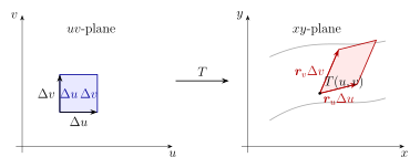
Remark 190 (Plain-language meaning). At a point $(u,v)$, the vectors \[\boldsymbol{r}_u=\left\langle x_u,\,y_u\right\rangle,\qquad \boldsymbol{r}_v=\left\langle x_v,\,y_v\right\rangle\] approximate how the map moves when you change $u$ or $v$ a little. A tiny $uv$-rectangle with sides $\Delta u$ and $\Delta v$ maps to a tiny parallelogram spanned by $\boldsymbol{r}_u\Delta u$ and $\boldsymbol{r}_v\Delta v$. Its area is approximately \[\big|\boldsymbol{r}_u\times \boldsymbol{r}_v\big| = \left|x_u y_v-x_v y_u\right| = \left|\frac{\partial(x,y)}{\partial(u,v)}\right|.\] So the Jacobian is a local area scale factor.

A small rectangle in the $uv$-plane maps to a small parallelogram in the $xy$-plane. The Jacobian gives the local area scaling.

6.1.3 Properties of Jacobians

Proposition 6.5 (Jacobian of a linear map). If \[x=au+bv,\qquad y=cu+dv,\] then \[\frac{\partial(x,y)}{\partial(u,v)}= \begin{vmatrix} a & b\\ c & d \end{vmatrix} =ad-bc.\] Geometrically, the unit square in $(u,v)$ maps to a parallelogram in $(x,y)$ with area $|ad-bc|$.

Proposition 6.6 (Inverse function and reciprocal Jacobian). If $T$ is one-to-one and differentiable with differentiable inverse $T^{-1}$, and if \[J(u,v)=\frac{\partial(x,y)}{\partial(u,v)}\neq 0,\] then the Jacobian of the inverse satisfies \[\begin{equation} \frac{\partial(u,v)}{\partial(x,y)}=\frac{1}{\frac{\partial(x,y)}{\partial(u,v)}} \end{equation}\] evaluated at corresponding points.

Proposition 6.7 (Jacobian of a composition). If $T:(u,v)\mapsto (x,y)$ and $S:(x,y)\mapsto (p,q)$ are differentiable, then \[\frac{\partial(p,q)}{\partial(u,v)} = \frac{\partial(p,q)}{\partial(x,y)}\, \frac{\partial(x,y)}{\partial(u,v)}.\]

Exercise 6.8. Let $T(u,v)=(x,y)=(u+2v,\,3u-v)$.

Compute $\dfrac{\partial(x,y)}{\partial(u,v)}$.
Find the area of the image of the rectangle $0\le u\le 2$, $0\le v\le 1$ under $T$.

6.2 Lesson 6.2: Double Integrals in General Coordinates

6.2.1 Change of Variables Theorem (Double Integrals)

Theorem 6.9 (Change of variables in $\mathbb{R}^2$). Let $T:(u,v)\mapsto (x,y)$ be a one-to-one $C^1$ transformation mapping a region $D^\ast$ in the $uv$-plane onto a region $D$ in the $xy$-plane. Assume the Jacobian \[J(u,v)=\frac{\partial(x,y)}{\partial(u,v)}\] is continuous and nonzero on $D^\ast$. If $f$ is continuous on $D$, then \[\begin{equation} \iint_D f(x,y)\,dA = \iint_{D^\ast} f(x(u,v),y(u,v))\,\left|J(u,v)\right|\,du\,dv. \end{equation}\]

Remark 196 (What the formula is saying). Replace $(x,y)$ by your formulas in terms of $(u,v)$, and multiply by the scale factor $\left|J\right|$. The absolute value is essential: even if the mapping flips orientation (negative Jacobian), physical area must remain positive.

6.2.2 Transforming Regions

Definition 6.11 (Image and preimage). If $D^\ast$ is a region in the $uv$-plane, its image is $D=T(D^\ast)$ in the $xy$-plane. Conversely, if $D$ is described naturally in $xy$, you try to find a transformation so that $D^\ast=T^{-1}(D)$ has simpler bounds.

Example 6.12 (Area of an ellipse via a scaling map). Let \[D=\left\{(x,y):\frac{x^2}{a^2}+\frac{y^2}{b^2}\le 1\right\},\qquad a>0,\ b>0.\] Use the substitution $x=au$, $y=bv$. Then \[\frac{x^2}{a^2}+\frac{y^2}{b^2}=u^2+v^2,\] so $D^\ast$ is the unit disk $u^2+v^2\le 1$. The Jacobian is \[\frac{\partial(x,y)}{\partial(u,v)}= \begin{vmatrix} a & 0\\ 0 & b \end{vmatrix} =ab.\] Therefore, \[\operatorname{Area}(D)=\iint_D 1\,dA =\iint_{D^\ast} 1\cdot |ab|\,du\,dv =ab\cdot \operatorname{Area}(D^\ast) =ab\cdot \pi =\pi ab.\]

Example 6.13 (A Gaussian-shaped integral on an ellipse). Let $D$ be the ellipse in Example 6.12 and consider \[I=\iint_D \exp\!\left(-\frac{x^2}{a^2}-\frac{y^2}{b^2}\right)\,dA.\] With $x=au$, $y=bv$, we have $\exp(-(x^2/a^2)-(y^2/b^2))=\exp(-(u^2+v^2))$ and $dA=|ab|\,du\,dv=ab\,du\,dv$. Hence \[I=ab\iint_{u^2+v^2\le 1} e^{-(u^2+v^2)}\,du\,dv.\] At this stage, switching to polar in the $uv$-plane finishes it: \[I=ab\int_{0}^{2\pi}\int_{0}^{1} e^{-r^2}\,r\,dr\,d\theta =ab\cdot 2\pi \cdot \left[-\frac12 e^{-r^2}\right]_{0}^{1} =ab\pi\,(1-e^{-1}).\]

6.2.3 Polar Coordinates as a Special Case

Proposition 6.14 (Polar Jacobian). Let \[x=r\cos\theta,\qquad y=r\sin\theta,\qquad r\ge 0.\] Then \[\frac{\partial(x,y)}{\partial(r,\theta)} = \begin{vmatrix} \cos\theta & -r\sin\theta\\ \sin\theta & r\cos\theta \end{vmatrix} =r(\cos^2\theta+\sin^2\theta)=r,\] so \[\begin{equation} dA=r\,dr\,d\theta. \end{equation}\]

Remark 201 (Practical cue). If you see circles, disks, annuli, or expressions like $x^2+y^2$, polar coordinates are usually the right tool because they turn $x^2+y^2$ into $r^2$ and simplify the region.

Exercise 6.16. Evaluate \[\iint_D (x^2+y^2)\,dA \quad\text{where}\quad D=\{(x,y):1\le x^2+y^2\le 4\}.\] Use polar coordinates and show each bound clearly.

6.3 Lesson 6.3: Cylindrical and Spherical Coordinates

6.3.1 Cylindrical Coordinates

Definition 6.17 (Cylindrical coordinates). Cylindrical coordinates represent points in $\mathbb{R}^3$ by $(r,\theta,z)$: \[x=r\cos\theta,\qquad y=r\sin\theta,\qquad z=z,\] with $r\ge 0$ and $\theta$ measured in the $xy$-plane.

Proposition 6.18 (Volume element in cylindrical coordinates). Under $(x,y,z)=(r\cos\theta,r\sin\theta,z)$, the Jacobian determinant is $r$, so \[\begin{equation} dV=r\,dr\,d\theta\,dz. \end{equation}\]

Example 6.19 (Volume of a right circular cylinder). Let $E=\{(x,y,z):x^2+y^2\le a^2,\ 0\le z\le h\}$. In cylindrical coordinates: \[0\le r\le a,\qquad 0\le \theta\le 2\pi,\qquad 0\le z\le h.\] Thus \[\operatorname{Vol}(E)=\iiint_E 1\,dV =\int_{0}^{h}\int_{0}^{2\pi}\int_{0}^{a} 1\cdot r\,dr\,d\theta\,dz =\int_{0}^{h}\left(2\pi\cdot \frac{a^2}{2}\right)dz =\pi a^2 h.\]

6.3.2 Spherical Coordinates

Definition 6.20 (Spherical coordinates). Spherical coordinates represent points in $\mathbb{R}^3$ by $(\rho,\phi,\theta)$: \[x=\rho\sin\phi\cos\theta,\qquad y=\rho\sin\phi\sin\theta,\qquad z=\rho\cos\phi,\] where $\rho\ge 0$ is distance from the origin, $0\le \phi\le \pi$ is the angle from the positive $z$-axis (polar angle), and $0\le \theta\le 2\pi$ is the angle in the $xy$-plane (azimuth).

Proposition 6.21 (Volume element in spherical coordinates). Under $(x,y,z)=(\rho\sin\phi\cos\theta,\allowbreak \rho\sin\phi\sin\theta,\allowbreak \rho\cos\phi)$, the Jacobian determinant is $\rho^2\sin\phi$, so \[\begin{equation} dV=\rho^2\sin\phi\,d\rho\,d\phi\,d\theta. \end{equation}\]

Remark 208 (Memory aid). In spherical, the volume scale has two effects:

$\rho^2$ because spheres grow like “radius squared” in surface area,
$\sin\phi$ because slices at polar angle $\phi$ have radius $\rho\sin\phi$ in the $xy$-direction.

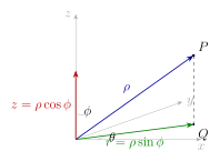
Cylindrical and spherical geometry: $r$ is the projection radius in the $xy$-plane, while $\rho$ is the full distance to the origin. Angles $\theta$ (azimuth) and $\phi$ (polar angle) locate direction.

6.3.3 Applications to Triple Integrals

Theorem 6.23 (Triple integrals in cylindrical coordinates). If a solid $E$ is described by bounds in $(r,\theta,z)$, then \[\iiint_E F(x,y,z)\,dV = \iiint_{E^\ast} F(r\cos\theta,r\sin\theta,z)\, r\,dr\,d\theta\,dz,\] with the bounds taken over the corresponding region $E^\ast$ in $(r,\theta,z)$-space.

Theorem 6.24 (Triple integrals in spherical coordinates). If a solid $E$ is described by bounds in $(\rho,\phi,\theta)$, then \[\iiint_E F(x,y,z)\,dV = \iiint_{E^\ast} F(\rho\sin\phi\cos\theta,\rho\sin\phi\sin\theta,\rho\cos\phi)\, \rho^2\sin\phi\,d\rho\,d\phi\,d\theta.\]

Example 6.25 (Volume of a ball). Compute the volume of the ball $\rho\le a$ (i.e. $x^2+y^2+z^2\le a^2$). In spherical coordinates: \[0\le \rho\le a,\qquad 0\le \phi\le \pi,\qquad 0\le \theta\le 2\pi.\] Thus \[\operatorname{Vol}=\iiint_E 1\,dV =\int_{0}^{2\pi}\int_{0}^{\pi}\int_{0}^{a} 1\cdot \rho^2\sin\phi\,d\rho\,d\phi\,d\theta =\left(\int_{0}^{2\pi}d\theta\right)\left(\int_{0}^{\pi}\sin\phi\,d\phi\right)\left(\int_{0}^{a}\rho^2\,d\rho\right).\] Compute each factor: \[\int_{0}^{2\pi}d\theta=2\pi,\qquad \int_{0}^{\pi}\sin\phi\,d\phi=\big[-\cos\phi\big]_{0}^{\pi}=2,\qquad \int_{0}^{a}\rho^2\,d\rho=\frac{a^3}{3}.\] Therefore $\operatorname{Vol}=\dfrac{4}{3}\pi a^3$.

Example 6.26 (A symmetric integral over a ball). Evaluate \[I=\iiint_{x^2+y^2+z^2\le a^2} (x^2+y^2+z^2)\,dV.\] In spherical, $x^2+y^2+z^2=\rho^2$, so \[I=\int_{0}^{2\pi}\int_{0}^{\pi}\int_{0}^{a} \rho^2\cdot \rho^2\sin\phi\,d\rho\,d\phi\,d\theta =\left(\int_{0}^{2\pi}d\theta\right)\left(\int_{0}^{\pi}\sin\phi\,d\phi\right)\left(\int_{0}^{a}\rho^4\,d\rho\right) =2\pi\cdot 2\cdot \frac{a^5}{5} =\frac{4\pi}{5}a^5.\]

Exercise 6.27. Set up (and evaluate) the integral for the volume inside the paraboloid $z=4-r^2$ and above the plane $z=0$ using cylindrical coordinates.

Exercise 6.28. Use spherical coordinates to compute the mass of the solid ball $x^2+y^2+z^2\le a^2$ with density $\rho(x,y,z)=k\sqrt{x^2+y^2+z^2}$, where $k>0$ is constant.

Chapter 6 Checklist

The Jacobian $\dfrac{\partial(x,y)}{\partial(u,v)}=x_u y_v-x_v y_u$ is the local area scale factor.
Change of variables for double integrals: \[\iint_D f(x,y)\,dA=\iint_{D^\ast} f(x(u,v),y(u,v))\left|\frac{\partial(x,y)}{\partial(u,v)}\right|\,du\,dv.\]
Polar is a special case: $dA=r\,dr\,d\theta$.
Cylindrical coordinates: $dV=r\,dr\,d\theta\,dz$.
Spherical coordinates: $dV=\rho^2\sin\phi\,d\rho\,d\phi\,d\theta$.

7 Chapter 7: Vector Calculus

Key Idea

Vector calculus connects geometry, differentiation, and integration in a powerful way.

A vector field assigns a vector to each point in space (think: wind velocity, fluid flow, force).
Line integrals measure accumulated work or circulation along a curve.
Flux integrals measure flow through a curve/surface.
The big theorems (Green, Stokes, Divergence) convert hard integrals into easier ones by swapping “boundary” and “interior.”

7.1 Lesson 7.1: Vector Fields

7.1.1 Definitions and Examples

Definition 7.1 (Vector field). A vector field on a region $D\subset\mathbb{R}^n$ is a function \[\boldsymbol{F}:D\to\mathbb{R}^n,\qquad \boldsymbol{F}(\boldsymbol{x})=\langle F_1(\boldsymbol{x}),\dots,F_n(\boldsymbol{x})\rangle.\] In $\mathbb{R}^2$, write $\boldsymbol{F}(x,y)=\langle P(x,y),Q(x,y)\rangle$. In $\mathbb{R}^3$, write $\boldsymbol{F}(x,y,z)=\langle P(x,y,z),Q(x,y,z),R(x,y,z)\rangle$.

Example 7.2 (Typical fields).

Radial field in $\mathbb{R}^2$: $\boldsymbol{F}(x,y)=\langle x,y\rangle$ (points away from the origin).
Rotational field in $\mathbb{R}^2$: $\boldsymbol{F}(x,y)=\langle -y,x\rangle$ (circles around the origin).
Inverse-square-type (away from origin) in $\mathbb{R}^3$: $\boldsymbol{F}=\dfrac{1}{(x^2+y^2+z^2)^{3/2}}\langle x,y,z\rangle$.

Remark 217 (Physical intuition). A vector field is a “vector at every point.” If it is velocity, field lines show how a particle would flow; if it is force, field lines show force directions.

7.1.2 Gradient Fields and Potential Functions

Definition 7.4 (Gradient field / conservative field). A vector field $\boldsymbol{F}$ on a region $D\subset\mathbb{R}^n$ is conservative (or a gradient field) if there exists a scalar function $f$ such that \[\boldsymbol{F}=\nabla f.\] The function $f$ is called a potential function for $\boldsymbol{F}$.

Example 7.5 (A gradient field). Let $f(x,y)=x^2y+y^3$. Then \[\nabla f=\langle 2xy,\ x^2+3y^2\rangle.\] So $\boldsymbol{F}(x,y)=\langle 2xy,\ x^2+3y^2\rangle$ is conservative on $\mathbb{R}^2$.

7.1.3 Visualizing Vector Fields (Sketching)

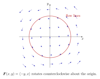
A rotational vector field in $\mathbb{R}^2$: arrows circulate around the origin.

Exercise 7.6. For $\boldsymbol{F}(x,y)=\langle x, -y\rangle$, describe qualitatively how the arrows point in each quadrant. Is the field more like “source/sink” or “rotation”?

7.2 Lesson 7.2: Line Integrals

7.2.1 Line Integrals of Scalar Functions

Definition 7.7 (Line integral of a scalar function). Let $C$ be a smooth curve parametrized by $\boldsymbol{r}(t)$, $a\le t\le b$, and let $f$ be continuous on $C$. Then \[\begin{equation} \int_C f\,ds = \int_a^b f(\boldsymbol{r}(t))\,\left\lVert \boldsymbol{r}'(t)\right\rVert\,dt. \end{equation}\]

Remark 222 (Interpretation). $\int_C f\,ds$ adds up $f$ weighted by arc length. For example, if $f$ is density along a wire, then $\int_C f\,ds$ is total mass.

7.2.2 Line Integrals of Vector Fields (Work Integrals)

Definition 7.9 (Work / circulation line integral). Let $\boldsymbol{F}$ be a vector field and $C$ be a smooth curve oriented by $\boldsymbol{r}(t)$, $a\le t\le b$. Then \[\begin{equation} \int_C \boldsymbol{F}\cdot d\boldsymbol{r} = \int_a^b \boldsymbol{F}(\boldsymbol{r}(t))\cdot \boldsymbol{r}'(t)\,dt. \end{equation}\]

Remark 224 (Physics meaning). If $\boldsymbol{F}$ is force and $\boldsymbol{r}(t)$ is a path, then $\int_C \boldsymbol{F}\cdot d\boldsymbol{r}$ is the work done by the force along that path.

7.2.3 Basic Parametrization Examples

Example 7.11 (Scalar line integral on a circle). Let $C$ be the circle $x^2+y^2=4$ traversed once counterclockwise. Parameterize: \[\boldsymbol{r}(t)=\langle 2\cos t,\ 2\sin t\rangle,\qquad 0\le t\le 2\pi.\] Then $\left\lVert \boldsymbol{r}'(t)\right\rVert=\left\lVert \langle -2\sin t,\ 2\cos t\rangle\right\rVert=2$. For $f(x,y)=x^2+y^2$, we have $f(\boldsymbol{r}(t))=4$. Hence \[\int_C f\,ds=\int_0^{2\pi} 4\cdot 2\,dt = 16\pi.\]

Example 7.12 (Work integral). Let $\boldsymbol{F}(x,y)=\langle -y,x\rangle$ and let $C$ be the unit circle $x^2+y^2=1$ counterclockwise. Use $\boldsymbol{r}(t)=\langle \cos t,\sin t\rangle$, $0\le t\le 2\pi$. Then \[\boldsymbol{r}'(t)=\langle -\sin t,\ \cos t\rangle,\qquad \boldsymbol{F}(\boldsymbol{r}(t))=\langle -\sin t,\ \cos t\rangle.\] So \[\boldsymbol{F}(\boldsymbol{r}(t))\cdot \boldsymbol{r}'(t) =\langle -\sin t,\cos t\rangle\cdot \langle -\sin t,\cos t\rangle =\sin^2 t+\cos^2 t=1.\] Therefore \[\int_C \boldsymbol{F}\cdot d\boldsymbol{r}=\int_{0}^{2\pi}1\,dt=2\pi.\]

Exercise 7.13. Compute $\displaystyle \int_C (x+y)\,ds$ where $C$ is the line segment from $(0,0)$ to $(2,1)$. (Hint: parametrize $\boldsymbol{r}(t)=\langle 2t,t\rangle$, $0\le t\le 1$.)

7.3 Lesson 7.3: The Fundamental Theorem for Line Integrals

7.3.1 Path Independence and Conservative Fields

Theorem 7.14 (Fundamental Theorem for Line Integrals). Let $\boldsymbol{F}=\nabla f$ be a conservative vector field on a region $D$, and let $C$ be a smooth curve in $D$ from point $A$ to point $B$. Then \[\begin{equation} \int_C \boldsymbol{F}\cdot d\boldsymbol{r} = f(B)-f(A). \end{equation}\] In particular, the integral depends only on endpoints, not on the path.

Corollary 7.15 (Zero circulation on closed curves). If $\boldsymbol{F}=\nabla f$ and $C$ is a closed curve (start = end), then \[\oint_C \boldsymbol{F}\cdot d\boldsymbol{r} = 0.\]

Remark 230 (How to use it). If you can find a potential function $f$, you avoid parametrizing curves entirely: compute $f(B)-f(A)$ and you are done.

7.3.2 Characterizing Conservative Fields in $\mathbb{R}^2$

Theorem 7.17 (Curl test in $\mathbb{R}^2$ (simply connected domains)). Let $\boldsymbol{F}(x,y)=\langle P(x,y),Q(x,y)\rangle$ with continuous partial derivatives on a simply connected region $D\subset\mathbb{R}^2$. Then $\boldsymbol{F}$ is conservative on $D$ if and only if \[\begin{equation} \frac{\partial P}{\partial y}=\frac{\partial Q}{\partial x}\quad \text{everywhere on }D. \end{equation}\]

Remark 232 (Why “simply connected” matters). If the region has holes, a field can satisfy $\partial P/\partial y=\partial Q/\partial x$ and still fail to be globally conservative. Example: $\langle -y/(x^2+y^2),\ x/(x^2+y^2)\rangle$ on $\mathbb{R}^2\setminus\{(0,0)\}$ has nontrivial circulation around the origin.

7.3.3 Finding a Potential Function

Proposition 7.19 (How to find $f$ when $\boldsymbol{F}=\langle P,Q\rangle$ is conservative). Assume $f_x=P$ and $f_y=Q$.

Integrate $P$ with respect to $x$ to get $f(x,y)=\int P(x,y)\,dx + g(y)$.
Differentiate this expression with respect to $y$ and set it equal to $Q$ to determine $g'(y)$.
Integrate $g'(y)$ to get $g(y)$ and complete $f$ (up to an additive constant).

Example 7.20 (Using the FTLI). Let $\boldsymbol{F}(x,y)=\langle 2xy,\ x^2+3y^2\rangle$. We claim $\boldsymbol{F}$ is conservative on $\mathbb{R}^2$. Check: \[\frac{\partial P}{\partial y}=2x,\qquad \frac{\partial Q}{\partial x}=2x,\] so Theorem 7.17 holds and $D=\mathbb{R}^2$ is simply connected.

Find a potential $f$: \[f_x=2xy \implies f(x,y)=\int 2xy\,dx=x^2y+g(y).\] Differentiate: \[f_y=x^2+g'(y).\] Set $f_y=Q=x^2+3y^2$ gives $g'(y)=3y^2$, so $g(y)=y^3$. Thus \[f(x,y)=x^2y+y^3.\]

Now compute the work from $A=(0,1)$ to $B=(2,0)$ along any path: \[\int_C \boldsymbol{F}\cdot d\boldsymbol{r}=f(B)-f(A)=\big(2^2\cdot 0+0^3\big)-\big(0^2\cdot 1+1^3\big)=0-1=-1.\]

Exercise 7.21. Determine whether $\boldsymbol{F}(x,y)=\langle y\cos x,\ \sin x\rangle$ is conservative on $\mathbb{R}^2$. If it is, find a potential $f$ and compute $\int_C \boldsymbol{F}\cdot d\boldsymbol{r}$ from $(0,0)$ to $(\pi,1)$.

7.4 Lesson 7.4: Green’s Theorem

7.4.1 Circulation Form of Green’s Theorem

Theorem 7.22 (Green’s Theorem (circulation form)). Let $C$ be a positively oriented (counterclockwise), simple, closed, piecewise-smooth curve in the plane, and let $D$ be the region it encloses. If $\boldsymbol{F}=\langle P,Q\rangle$ has continuous partial derivatives on an open region containing $D$, then \[\begin{equation} \oint_C P\,dx+Q\,dy = \iint_D \left(\frac{\partial Q}{\partial x}-\frac{\partial P}{\partial y}\right)\,dA. \end{equation}\]

Remark 237 (What it does). A line integral around the boundary becomes a double integral over the interior. This is usually a huge simplification when the boundary is complicated but the interior is easy (or vice versa).

7.4.2 Flux Form of Green’s Theorem

Definition 7.24 (Outward unit normal in the plane). If $C$ is oriented counterclockwise with tangent direction $d\boldsymbol{r}=\langle dx,dy\rangle$, then an outward normal line element can be represented by \[\boldsymbol{n}\,ds=\langle dy,\ -dx\rangle.\]

Theorem 7.25 (Green’s Theorem (flux form)). With the same hypotheses as Theorem 7.22, we have \[\begin{equation} \oint_C \boldsymbol{F}\cdot \boldsymbol{n}\,ds = \oint_C P\,dy - Q\,dx = \iint_D \left(\frac{\partial P}{\partial x}+\frac{\partial Q}{\partial y}\right)\,dA. \end{equation}\]

Remark 240 (Divergence in 2D). The integrand $\dfrac{\partial P}{\partial x}+\dfrac{\partial Q}{\partial y}$ is the 2D divergence. The flux form says: total outward flux through the boundary equals the integral of divergence over the region.

7.4.3 Applications

Example 7.27 (Compute area using Green’s Theorem). Take $P=-\dfrac{y}{2}$ and $Q=\dfrac{x}{2}$. Then \[\frac{\partial Q}{\partial x}-\frac{\partial P}{\partial y} =\frac12-\left(-\frac12\right)=1.\] By Theorem 7.22, \[\oint_C \left(-\frac{y}{2}\,dx+\frac{x}{2}\,dy\right) =\iint_D 1\,dA=\operatorname{Area}(D).\] So \[\begin{equation} \operatorname{Area}(D)=\frac12\oint_C (x\,dy-y\,dx). \end{equation}\]

Example 7.28 (Work around a circle quickly). Let $\boldsymbol{F}=\langle -y,x\rangle$ and let $C$ be the unit circle oriented counterclockwise. In Example 7.12 we computed the circulation as $2\pi$ by parametrization. Now use Green: \[\frac{\partial Q}{\partial x}-\frac{\partial P}{\partial y} =\frac{\partial}{\partial x}(x)-\frac{\partial}{\partial y}(-y)=1-(-1)=2.\] Hence \[\oint_C P\,dx+Q\,dy=\iint_D 2\,dA=2\cdot \operatorname{Area}(\text{unit disk})=2\cdot \pi=2\pi,\] agreeing with the earlier result.

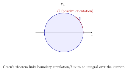
A positively oriented boundary curve $C$ enclosing a region $D$.

Exercise 7.29. Use Green’s Theorem to compute \[\oint_C (x^2-y^2)\,dx + 2xy\,dy\] where $C$ is the positively oriented circle $x^2+y^2=1$.

7.5 Lesson 7.5: Curl and Divergence

7.5.1 Definitions in $\mathbb{R}^3$

Definition 7.30 (Divergence). For a $C^1$ vector field $\boldsymbol{F}=\langle P,Q,R\rangle$ on $\mathbb{R}^3$, the divergence is \[\nabla\cdot \boldsymbol{F} = P_x+Q_y+R_z.\]

Definition 7.31 (Curl). For a $C^1$ vector field $\boldsymbol{F}=\langle P,Q,R\rangle$ on $\mathbb{R}^3$, the curl is \[\nabla\times \boldsymbol{F} = \left\langle R_y-Q_z,\ P_z-R_x,\ Q_x-P_y \right\rangle.\]

Remark 246 (Interpretation). Divergence measures “net outflow per unit volume” (sources/sinks). Curl measures “local rotation” (circulation density).

7.5.2 Key Identities

Proposition 7.33 (Always true identities). If $f$ is $C^2$ and $\boldsymbol{F}$ is $C^2$, then \[\nabla\times(\nabla f)=\boldsymbol{0}, \qquad \nabla\cdot(\nabla\times \boldsymbol{F})=0.\]

Remark 248 (A practical consequence). If $\boldsymbol{F}$ is a gradient field ($\boldsymbol{F}=\nabla f$), then $\nabla\times \boldsymbol{F}=\boldsymbol{0}$. This is a necessary condition for being conservative; in simply connected regions it is also sufficient.

7.5.3 Examples

Example 7.35 (Compute divergence and curl). Let $\boldsymbol{F}(x,y,z)=\langle x^2y,\ yz,\ xz^2\rangle$. Then \[\nabla\cdot \boldsymbol{F} =\frac{\partial}{\partial x}(x^2y)+\frac{\partial}{\partial y}(yz)+\frac{\partial}{\partial z}(xz^2) =2xy+z+2xz.\] Also \[\begin{align*} \nabla\times \boldsymbol{F} &= \left\langle R_y-Q_z,\ P_z-R_x,\ Q_x-P_y \right\rangle \\[8pt] &= \begin{bmatrix} \dfrac{\partial}{\partial y}(xz^2)-\dfrac{\partial}{\partial z}(yz) \\[8pt] \dfrac{\partial}{\partial z}(x^2y)-\dfrac{\partial}{\partial x}(xz^2) \\[8pt] \dfrac{\partial}{\partial x}(yz)-\dfrac{\partial}{\partial y}(x^2y) \end{bmatrix}^T \\[8pt] &= \langle 0-y,\ 0-z^2,\ 0-x^2 \rangle \\[5pt] &= \langle -y,\ -z^2,\ -x^2\rangle. \end{align*}\]

Exercise 7.36. Let $\boldsymbol{F}=\langle yz,\ xz,\ xy\rangle$.

Compute $\nabla\cdot \boldsymbol{F}$.
Compute $\nabla\times \boldsymbol{F}$.
Is $\boldsymbol{F}$ conservative on $\mathbb{R}^3$? (Justify.)

7.6 Lesson 7.6: Stokes’ Theorem and the Divergence Theorem

7.6.1 Stokes’ Theorem

Theorem 7.37 (Stokes’ Theorem). Let $S$ be an oriented, smooth surface with boundary curve $\partial S=C$ (a closed curve). Let $\boldsymbol{n}$ be the unit normal consistent with the positive orientation of $C$ (right-hand rule). If $\boldsymbol{F}$ has continuous partial derivatives on an open region containing $S$, then \[\begin{equation} \oint_{C} \boldsymbol{F}\cdot d\boldsymbol{r} = \iint_{S} (\nabla\times \boldsymbol{F})\cdot \boldsymbol{n}\,dS. \end{equation}\]

Remark 252 (Meaning). A circulation integral around the boundary equals the flux of curl through the surface. It is the 3D analogue of Green’s theorem.

Example 7.39 (A simple Stokes computation: choose the easiest surface). Let $\boldsymbol{F}=\langle -y,x,0\rangle$ and let $C$ be the circle $x^2+y^2=1$ in the plane $z=0$ oriented counterclockwise (viewed from $+z$). Choose $S$ to be the unit disk in the plane $z=0$ with upward normal $\boldsymbol{n}=\langle 0,0,1\rangle$.

Compute curl: \[\nabla\times \boldsymbol{F} = \left\langle 0-0,\ 0-0,\ \frac{\partial}{\partial x}(x)-\frac{\partial}{\partial y}(-y) \right\rangle = \langle 0,0,2\rangle.\] Then \[\iint_S (\nabla\times \boldsymbol{F})\cdot \boldsymbol{n}\,dS = \iint_S 2\,dS =2\cdot \operatorname{Area}(\text{unit disk}) =2\pi.\] Hence, by Stokes, \[\oint_C \boldsymbol{F}\cdot d\boldsymbol{r} =2\pi,\] matching Chapter 7 line-integral computations.

7.6.2 Divergence Theorem

Theorem 7.40 (Divergence Theorem (Gauss)). Let $E$ be a solid region in $\mathbb{R}^3$ with closed, piecewise-smooth boundary surface $S=\partial E$ oriented outward. If $\boldsymbol{F}$ has continuous partial derivatives on an open region containing $E$, then \[\begin{equation} \iint_{S} \boldsymbol{F}\cdot \boldsymbol{n}\,dS = \iiint_{E} (\nabla\cdot \boldsymbol{F})\,dV. \end{equation}\]

Remark 255 (Meaning). Total outward flux through the boundary equals total divergence inside the volume. This is the 3D analogue of the flux form of Green’s theorem.

7.6.3 Applications

Example 7.42 (Flux through a sphere using divergence theorem). Let $\boldsymbol{F}=\langle x,y,z\rangle$ and let $S$ be the sphere $x^2+y^2+z^2=a^2$ oriented outward. Then \[\nabla\cdot \boldsymbol{F} = 1+1+1=3.\] Let $E$ be the ball $x^2+y^2+z^2\le a^2$. By Theorem 7.40, \[\iint_S \boldsymbol{F}\cdot \boldsymbol{n}\,dS=\iiint_E 3\,dV=3\cdot \operatorname{Vol}(E)=3\cdot \frac{4}{3}\pi a^3=4\pi a^3.\]

Example 7.43 (Why conservative fields have zero circulation on closed curves). If $\boldsymbol{F}=\nabla f$ is $C^2$, then $\nabla\times \boldsymbol{F}=\nabla\times(\nabla f)=\boldsymbol{0}$ by Proposition 7.33. By Stokes’ theorem Theorem 7.37, \[\oint_C \boldsymbol{F}\cdot d\boldsymbol{r}=\iint_S (\nabla\times \boldsymbol{F})\cdot \boldsymbol{n}\,dS=\iint_S 0\,dS=0.\] This recovers the “closed curve integral is zero” fact in a broader 3D setting.

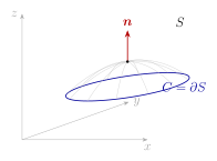
Stokes’ theorem relates a line integral around $C=\partial S$ to the flux of $\nabla\times \boldsymbol{F}$ through the surface $S$.

Exercise 7.44. Let $\boldsymbol{F}=\langle y,-x,0\rangle$ and let $C$ be the circle $x^2+y^2=4$ in the plane $z=3$, oriented counterclockwise when viewed from above. Use Stokes’ theorem to compute $\displaystyle \oint_C \boldsymbol{F}\cdot d\boldsymbol{r}$ by choosing a convenient surface.

Exercise 7.45. Use the divergence theorem to compute the outward flux of $\boldsymbol{F}=\langle x^3,y^3,z^3\rangle$ across the boundary of the cube $0\le x,y,z\le 1$.

Chapter 7 Checklist

Vector fields $\boldsymbol{F}=\langle P,Q\rangle$ (2D) or $\langle P,Q,R\rangle$ (3D) model flow/force.
Scalar line integral: $\displaystyle \int_C f\,ds=\int_a^b f(\boldsymbol{r}(t))\|\boldsymbol{r}'(t)\|\,dt$.
Work integral: $\displaystyle \int_C \boldsymbol{F}\cdot d\boldsymbol{r}=\int_a^b \boldsymbol{F}(\boldsymbol{r}(t))\cdot \boldsymbol{r}'(t)\,dt$.
Fundamental Theorem for Line Integrals: if $\boldsymbol{F}=\nabla f$, then $\int_C \boldsymbol{F}\cdot d\boldsymbol{r}=f(B)-f(A)$.
Green’s theorem: boundary circulation/flux $\leftrightarrow$ interior double integral.
Divergence $\nabla\cdot \boldsymbol{F}=P_x+Q_y+R_z$ and curl $\nabla\times \boldsymbol{F}=\langle R_y-Q_z,\ P_z-R_x,\ Q_x-P_y\rangle$.
Stokes: $\displaystyle \oint_{\partial S} \boldsymbol{F}\cdot d\boldsymbol{r}=\iint_S (\nabla\times \boldsymbol{F})\cdot \boldsymbol{n}\,dS$.
Divergence theorem: $\displaystyle \iint_{\partial E}\boldsymbol{F}\cdot \boldsymbol{n}\,dS=\iiint_E (\nabla\cdot \boldsymbol{F})\,dV$.

8 Chapter 8: Parametric Surfaces and Surface Integrals

Key Idea

Curves are 1-dimensional objects, so we integrate along them with $ds$ or $d\boldsymbol{r}$. Surfaces are 2-dimensional objects, so we integrate over them with an area element $dS$.

The key geometric fact is: a smooth surface can be parameterized by two variables $(u,v)$, and the tiny surface patch area is controlled by the cross product \[\bigl\|\boldsymbol{r}_u\times \boldsymbol{r}_v\bigr\|.\] That single quantity drives both surface area and surface integrals (scalar and flux).

8.1 Lesson 8.1: Parametric Surfaces

8.1.1 Parametrizations and Tangent Planes

Definition 8.1 (Parametric surface). A parametric surface is a vector-valued function \[\boldsymbol{r}(u,v)=\langle x(u,v),\,y(u,v),\,z(u,v)\rangle,\] defined on a region $D^\ast\subset \mathbb{R}^2$ (the parameter domain). The image \[S=\{\boldsymbol{r}(u,v):(u,v)\in D^\ast\}\subset\mathbb{R}^3\] is the surface.

Definition 8.2 (Tangent vectors and normal). If $\boldsymbol{r}$ has continuous partial derivatives, then the vectors \[\boldsymbol{r}_u=\frac{\partial \boldsymbol{r}}{\partial u},\qquad \boldsymbol{r}_v=\frac{\partial \boldsymbol{r}}{\partial v}\] are tangent to the surface (they point along the $u$- and $v$-coordinate curves). If $\boldsymbol{r}_u\times \boldsymbol{r}_v\neq \boldsymbol{0}$, then a normal vector to the surface is \[\boldsymbol{n} = \boldsymbol{r}_u\times \boldsymbol{r}_v.\]

Proposition 8.3 (Tangent plane to a parametric surface). At a point $\boldsymbol{r}(u_0,v_0)$ with $\boldsymbol{r}_u\times \boldsymbol{r}_v\neq\boldsymbol{0}$, the tangent plane is the plane through $\boldsymbol{r}(u_0,v_0)$ with normal $\boldsymbol{n}=\boldsymbol{r}_u(u_0,v_0)\times \boldsymbol{r}_v(u_0,v_0)$: \[\boldsymbol{n}\cdot\bigl(\langle x,y,z\rangle-\boldsymbol{r}(u_0,v_0)\bigr)=0.\]

Remark 263 (Plain-language picture). A surface is locally like a stretched sheet. The vectors $\boldsymbol{r}_u$ and $\boldsymbol{r}_v$ span the local directions you can move while staying on the sheet. Their cross product points perpendicular to the sheet.

Example 8.5 (A plane as a parametric surface). The plane $z=1+x+2y$ can be parameterized by letting $u=x$ and $v=y$: \[\boldsymbol{r}(u,v)=\langle u,\ v,\ 1+u+2v\rangle,\qquad (u,v)\in\mathbb{R}^2.\] Then \[\boldsymbol{r}_u=\langle 1,0,1\rangle,\qquad \boldsymbol{r}_v=\langle 0,1,2\rangle,\] so a normal is \[\boldsymbol{r}_u\times\boldsymbol{r}_v= \begin{vmatrix} \boldsymbol{i} & \boldsymbol{j} & \boldsymbol{k}\\ 1&0&1\\ 0&1&2 \end{vmatrix} =\langle -1,-2,1\rangle.\]

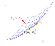
A surface patch with two tangent directions and a normal direction at a point.

Exercise 8.6. Parameterize the cylinder $x^2+y^2=9$ for $0\le z\le 2$ using $(\theta,z)$, and compute $\boldsymbol{r}_\theta\times \boldsymbol{r}_z$.

8.2 Lesson 8.2: Surface Area

8.2.1 Surface Area of a Parametric Surface

Theorem 8.7 (Surface area formula). Let $S$ be parametrized by $\boldsymbol{r}(u,v)$ on a region $D^\ast$ and assume $\boldsymbol{r}_u\times \boldsymbol{r}_v$ is continuous and nonzero on $D^\ast$. Then the surface area is \[\begin{equation} \operatorname{Area}(S)=\iint_{D^\ast}\bigl\|\boldsymbol{r}_u\times \boldsymbol{r}_v\bigr\|\,du\,dv. \end{equation}\]

Remark 267 (What $\|\boldsymbol{r}_u\times \boldsymbol{r}_v\|$ is doing). In the parameter domain, a tiny rectangle has area $du\,dv$. On the surface, it becomes a tiny parallelogram spanned by $\boldsymbol{r}_u\,du$ and $\boldsymbol{r}_v\,dv$, whose area is $\|\boldsymbol{r}_u\times \boldsymbol{r}_v\|\,du\,dv$. Integrating adds them up.

8.2.2 Graph Surfaces: $z=g(x,y)$

Proposition 8.9 (Surface area element for a graph). If $S$ is the graph $z=g(x,y)$ over a region $D$ in the $xy$-plane, and $g_x,g_y$ are continuous on $D$, then \[\begin{equation} dS=\sqrt{1+g_x(x,y)^2+g_y(x,y)^2}\,dA. \end{equation}\] Hence \[\operatorname{Area}(S)=\iint_D \sqrt{1+g_x^2+g_y^2}\,dA.\]

Example 8.10 (Surface area of a paraboloid patch). Find the area of the surface $z=x^2+y^2$ above the disk $x^2+y^2\le R^2$.

Here $g_x=2x$ and $g_y=2y$, so by Proposition 8.9, \[dS=\sqrt{1+4x^2+4y^2}\,dA=\sqrt{1+4r^2}\,dA\] in polar coordinates. Thus \[\operatorname{Area} =\int_{0}^{2\pi}\int_{0}^{R}\sqrt{1+4r^2}\,r\,dr\,d\theta.\] Compute the $r$-integral. Let $u=1+4r^2$, so $du=8r\,dr$ and $r\,dr=\frac{1}{8}du$: \[\int_0^R r\sqrt{1+4r^2}\,dr =\frac{1}{8}\int_{1}^{1+4R^2} u^{1/2}\,du =\frac{1}{8}\cdot \frac{2}{3}\Big[u^{3/2}\Big]_{1}^{1+4R^2} =\frac{1}{12}\left((1+4R^2)^{3/2}-1\right).\] Therefore \[\operatorname{Area} =2\pi\cdot \frac{1}{12}\left((1+4R^2)^{3/2}-1\right) =\frac{\pi}{6}\left((1+4R^2)^{3/2}-1\right).\]

Example 8.11 (Surface area of a sphere). Parameterize the sphere of radius $a>0$ by spherical angles: \[\boldsymbol{r}(\phi,\theta)=\langle a\sin\phi\cos\theta,\ a\sin\phi\sin\theta,\ a\cos\phi\rangle, \qquad 0\le \phi\le \pi,\ 0\le\theta\le 2\pi.\] Compute partial derivatives: \[\boldsymbol{r}_\phi=\langle a\cos\phi\cos\theta,\ a\cos\phi\sin\theta,\ -a\sin\phi\rangle,\qquad \boldsymbol{r}_\theta=\langle -a\sin\phi\sin\theta,\ a\sin\phi\cos\theta,\ 0\rangle.\] A direct computation gives \[\bigl\|\boldsymbol{r}_\phi\times \boldsymbol{r}_\theta\bigr\|=a^2\sin\phi.\] Therefore, by Theorem 8.7, \[\operatorname{Area}(S) =\int_{0}^{2\pi}\int_{0}^{\pi} a^2\sin\phi\,d\phi\,d\theta =a^2\left(\int_{0}^{2\pi}d\theta\right)\left(\int_{0}^{\pi}\sin\phi\,d\phi\right) =a^2(2\pi)(2)=4\pi a^2.\]

Exercise 8.12. Use Proposition 8.9 to set up the surface area of $z=xy$ over the rectangle $0\le x\le 1$, $0\le y\le 2$. (You do not need to evaluate the integral.)

8.3 Lesson 8.3: Surface Integrals of Scalar Fields

8.3.1 Definition

Definition 8.13 (Surface integral of a scalar function). Let $S$ be a smooth surface and let $f$ be continuous on $S$. The surface integral of $f$ over $S$ is denoted \[\iint_S f\,dS.\] If $S$ is parametrized by $\boldsymbol{r}(u,v)$ on $D^\ast$, then \[\begin{equation} \iint_S f\,dS = \iint_{D^\ast} f(\boldsymbol{r}(u,v))\,\bigl\|\boldsymbol{r}_u\times \boldsymbol{r}_v\bigr\|\,du\,dv. \end{equation}\]

Remark 273 (Interpretation). $\iint_S f\,dS$ adds up $f$ weighted by surface area. If $f$ is a surface density (mass per unit area), then $\iint_S f\,dS$ is total mass of a thin shell.

8.3.2 Graph Case

Proposition 8.15 (Scalar surface integral over a graph). If $S$ is $z=g(x,y)$ over a region $D$ in the $xy$-plane, then \[\begin{equation} \iint_S f\,dS = \iint_D f(x,y,g(x,y))\,\sqrt{1+g_x^2+g_y^2}\,dA. \end{equation}\]

Example 8.16 (A clean computation on a plane). Let $S$ be the part of the plane $z=1+x+y$ above the unit square $D=\{(x,y):0\le x\le 1,\ 0\le y\le 1\}$, and let $f(x,y,z)=z$.

Here $g(x,y)=1+x+y$, so $g_x=1$ and $g_y=1$. Thus \[\sqrt{1+g_x^2+g_y^2}=\sqrt{1+1+1}=\sqrt{3}.\] By Proposition 8.15, \[\iint_S z\,dS =\iint_D (1+x+y)\sqrt{3}\,dA =\sqrt{3}\int_{0}^{1}\int_{0}^{1}(1+x+y)\,dy\,dx.\] Compute: \[\int_{0}^{1}(1+x+y)\,dy=(1+x)\cdot 1+\frac12=\frac32+x, \qquad \int_{0}^{1}\left(\frac32+x\right)\,dx=\frac32+\frac12=2.\] Therefore \[\iint_S z\,dS = 2\sqrt{3}.\]

Exercise 8.17. Let $S$ be the hemisphere $x^2+y^2+z^2=1$ with $z\ge 0$ and let $f(x,y,z)=z$. Write $\iint_S f\,dS$ using a spherical parametrization. (You do not need to evaluate.)

8.4 Lesson 8.4: Surface Integrals of Vector Fields (Flux)

8.4.1 Oriented Surfaces and Flux

Definition 8.18 (Oriented surface). A smooth surface $S$ is oriented if we choose a continuous unit normal vector $\boldsymbol{n}$ at each point of $S$. For a closed surface, the standard orientation is outward. For a graph $z=g(x,y)$, a common choice is upward (positive $z$-component).

Definition 8.19 (Flux integral). Let $\boldsymbol{F}$ be a vector field and let $S$ be an oriented surface with unit normal $\boldsymbol{n}$. The flux of $\boldsymbol{F}$ through $S$ is \[\begin{equation} \iint_S \boldsymbol{F}\cdot \boldsymbol{n}\,dS. \end{equation}\]

Remark 279 (Plain-language meaning). $\boldsymbol{F}\cdot \boldsymbol{n}$ measures how much the field points through the surface (perpendicular component). Integrating adds up that “through-flow” over the entire surface.

8.4.2 Flux Using a Parametrization

Proposition 8.21 (Flux via $\boldsymbol{r}_u\times \boldsymbol{r}_v$). If $S$ is parametrized by $\boldsymbol{r}(u,v)$ on $D^\ast$ and oriented consistently with the normal \[\boldsymbol{n}\,dS = \bigl(\boldsymbol{r}_u\times \boldsymbol{r}_v\bigr)\,du\,dv,\] then \[\begin{equation} \iint_S \boldsymbol{F}\cdot \boldsymbol{n}\,dS = \iint_{D^\ast} \boldsymbol{F}(\boldsymbol{r}(u,v))\cdot\bigl(\boldsymbol{r}_u\times \boldsymbol{r}_v\bigr)\,du\,dv. \end{equation}\] If the opposite orientation is required, replace $\boldsymbol{r}_u\times \boldsymbol{r}_v$ by its negative.

8.4.3 Flux Through a Graph Surface

Proposition 8.22 (Flux for a graph $z=g(x,y)$). Let $S$ be the graph $z=g(x,y)$ over a region $D$ in the $xy$-plane. A parametrization is $\boldsymbol{r}(x,y)=\langle x,y,g(x,y)\rangle$. Then \[\boldsymbol{r}_x=\langle 1,0,g_x\rangle,\qquad \boldsymbol{r}_y=\langle 0,1,g_y\rangle, \qquad \boldsymbol{r}_x\times\boldsymbol{r}_y=\langle -g_x,-g_y,1\rangle.\] For the upward orientation (positive $z$-component), we have \[\begin{equation} \iint_S \boldsymbol{F}\cdot \boldsymbol{n}\,dS = \iint_D \boldsymbol{F}(x,y,g(x,y))\cdot \langle -g_x,-g_y,1\rangle\,dA. \end{equation}\] For the downward orientation, use the negative of this vector.

Example 8.23 (A flux integral that collapses nicely). Let $\boldsymbol{F}=\langle x,y,z\rangle$, and let $S$ be the part of the plane \[z=2-x-y\] above the triangle $D=\{(x,y): x\ge 0,\ y\ge 0,\ x+y\le 1\}$, oriented upward.

Here $g(x,y)=2-x-y$, so $g_x=-1$ and $g_y=-1$. By Proposition 8.22, \[\boldsymbol{n}\,dS=\langle -g_x,-g_y,1\rangle\,dA=\langle 1,1,1\rangle\,dA.\] Also \[\boldsymbol{F}(x,y,g)=\langle x,\ y,\ 2-x-y\rangle, \quad\Rightarrow\quad \boldsymbol{F}\cdot \langle 1,1,1\rangle = x+y+(2-x-y)=2.\] Therefore the flux is \[\iint_S \boldsymbol{F}\cdot \boldsymbol{n}\,dS = \iint_D 2\,dA =2\cdot \operatorname{Area}(D).\] The triangle $D$ has legs of length $1$ and $1$, so $\operatorname{Area}(D)=\frac12$. Hence the flux is \[\iint_S \boldsymbol{F}\cdot \boldsymbol{n}\,dS = 1.\]

Exercise 8.24. Let $\boldsymbol{F}=\langle 0,0,z\rangle$ and let $S$ be the graph $z=x^2+y^2$ over the disk $x^2+y^2\le 1$, oriented upward. Set up $\iint_S \boldsymbol{F}\cdot \boldsymbol{n}\,dS$ using Proposition 8.22, and simplify the integrand as much as possible.

8.5 Lesson 8.5: Orientation, Boundaries, and Strategy

8.5.1 Orientation Conventions

Remark 284 (Right-hand rule). If a surface $S$ has boundary curve $C=\partial S$ and $S$ is oriented by $\boldsymbol{n}$, then the positive orientation of $C$ is given by the right-hand rule: curling the fingers of your right hand in the direction of $C$, your thumb points in the direction of $\boldsymbol{n}$.

8.5.2 Choosing the Best Method

Proposition 8.26 (Workflow for surface integrals). To compute surface area or a surface integral:

Decide whether the surface is best described as a graph $z=g(x,y)$ or a parametric surface $\boldsymbol{r}(u,v)$.
For area or scalar surface integrals, compute the factor $\|\boldsymbol{r}_u\times\boldsymbol{r}_v\|$ (or $\sqrt{1+g_x^2+g_y^2}$).
For flux, compute the oriented normal element $\boldsymbol{n}\,dS$: \[\boldsymbol{n}\,dS = (\boldsymbol{r}_u\times \boldsymbol{r}_v)\,du\,dv \quad\text{or}\quad \boldsymbol{n}\,dS=\langle -g_x,-g_y,1\rangle\,dA\] with the correct sign for orientation.
Translate the region into clean bounds in the parameter domain (often polar/cylindrical is the cleanest).

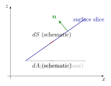
Schematic idea: $dS$ (surface element) is larger than its projection $dA$ when the surface tilts; the factor $\sqrt{1+g_x^2+g_y^2}$ measures the tilt.

Exercise 8.27. A surface is given parametrically by $\boldsymbol{r}(u,v)=\langle u,\ v,\ uv\rangle$ on $0\le u\le 1$, $0\le v\le 2$.

Compute $\|\boldsymbol{r}_u\times \boldsymbol{r}_v\|$.
Set up the surface area integral.
Set up $\iint_S z\,dS$.

Chapter 8 Checklist

Parametric surface: $\boldsymbol{r}(u,v)$; tangent vectors $\boldsymbol{r}_u,\boldsymbol{r}_v$; normal $\boldsymbol{r}_u\times \boldsymbol{r}_v$.
Surface area: $\displaystyle \operatorname{Area}(S)=\iint_{D^\ast}\|\boldsymbol{r}_u\times\boldsymbol{r}_v\|\,du\,dv$.
Graph surface $z=g(x,y)$: $\displaystyle dS=\sqrt{1+g_x^2+g_y^2}\,dA$.
Scalar surface integral: $\displaystyle \iint_S f\,dS=\iint_{D^\ast} f(\boldsymbol{r}(u,v))\|\boldsymbol{r}_u\times\boldsymbol{r}_v\|\,du\,dv$.
Flux integral: $\displaystyle \iint_S \boldsymbol{F}\cdot\boldsymbol{n}\,dS=\iint_{D^\ast}\boldsymbol{F}(\boldsymbol{r}(u,v))\cdot(\boldsymbol{r}_u\times\boldsymbol{r}_v)\,du\,dv$ (orientation matters).
For graphs, upward flux uses $\langle -g_x,-g_y,1\rangle\,dA$.

9 Chapter 9: The Big Theorems of Vector Calculus

Key Idea

Vector calculus has three “bridge theorems” that convert difficult integrals into easier ones:

Green’s Theorem (2D): boundary line integral $\leftrightarrow$ interior double integral.
Stokes’ Theorem (3D): boundary circulation $\leftrightarrow$ surface integral of curl.
Divergence Theorem (3D): surface flux $\leftrightarrow$ volume integral of divergence.

They all share the same philosophy: what happens on the boundary is controlled by what happens inside.

9.1 Lesson 9.1: A Unifying View (Orientation and Boundaries)

9.1.1 Orientation in 2D and 3D

Remark 287 (Orientation is not optional). Each theorem requires a consistent orientation:

In the plane, positive orientation means the boundary curve is traversed counterclockwise.
In space, the right-hand rule ties the orientation of a boundary curve $\partial S$ to the chosen normal on the surface $S$.
For closed surfaces, the standard is outward orientation.

If you flip the orientation, the integral changes sign.

9.1.2 A Quick “Boundary-of-a-Boundary” Principle

Proposition 9.2 (Boundary of a boundary is empty). Informally, $\partial(\partial S)=\varnothing$. In practice: if you take a surface boundary curve $C=\partial S$, then $C$ has no boundary endpoints because it is a closed loop. This principle underlies why “curl of a gradient” and “divergence of a curl” vanish.

Remark 289 (What to remember). The big theorems are “consistent bookkeeping” rules for how derivatives measure interior behavior and integrals measure accumulated boundary behavior.

9.2 Lesson 9.2: Green’s Theorem (Both Forms and Consequences)

9.2.1 Statements

Theorem 9.4 (Green’s Theorem: circulation form). Let $C$ be a positively oriented, simple, closed, piecewise-smooth curve in the plane, and let $D$ be the region it encloses. If $\boldsymbol{F}=\langle P,Q\rangle$ has continuous partial derivatives on an open set containing $D$, then \[\begin{equation} \oint_C P\,dx+Q\,dy = \iint_D \left(\frac{\partial Q}{\partial x}-\frac{\partial P}{\partial y}\right)\,dA. \end{equation}\]

Theorem 9.5 (Green’s Theorem: flux form). Under the same hypotheses, \[\begin{equation} \oint_C \boldsymbol{F}\cdot \boldsymbol{n}\,ds = \oint_C P\,dy - Q\,dx = \iint_D \left(\frac{\partial P}{\partial x}+\frac{\partial Q}{\partial y}\right)\,dA. \end{equation}\]

Remark 292 (Two key operators in 2D). \[\text{2D curl (scalar)}:\quad \frac{\partial Q}{\partial x}-\frac{\partial P}{\partial y}, \qquad \text{2D divergence}:\quad \frac{\partial P}{\partial x}+\frac{\partial Q}{\partial y}.\] Green’s theorem converts boundary circulation/flux into interior integrals of these quantities.

9.2.2 Consequences

Corollary 9.7 (Area formula). If $C=\partial D$ is positively oriented, then \[\begin{equation} \operatorname{Area}(D)=\frac12\oint_C (x\,dy-y\,dx). \end{equation}\]

Proof. Take $P=-y/2$ and $Q=x/2$. Then $Q_x-P_y=1$ and apply Theorem 9.4. ◻

Corollary 9.8 (Circulation is zero for conservative fields). If $\boldsymbol{F}=\nabla f$ on a region containing $D$, then \[\oint_C \boldsymbol{F}\cdot d\boldsymbol{r}=0.\]

Proof. If $\boldsymbol{F}=\langle P,Q\rangle=\nabla f$, then $P=f_x$ and $Q=f_y$, so $Q_x-P_y=f_{yx}-f_{xy}=0$ (Clairaut). Apply Theorem 9.4. ◻

9.2.3 Worked Example

Example 9.9 (Use Green instead of parametrizing). Compute $\displaystyle \oint_C (x^2-y^2)\,dx + 2xy\,dy$ where $C$ is the circle $x^2+y^2=4$ oriented counterclockwise.

Here $P=x^2-y^2$ and $Q=2xy$. Then \[\frac{\partial Q}{\partial x}-\frac{\partial P}{\partial y}=2y-(-2y)=4y.\] So by Theorem 9.4, \[\oint_C P\,dx+Q\,dy=\iint_D 4y\,dA,\] where $D$ is the disk $x^2+y^2\le 4$. The integrand $4y$ is odd in $y$ and the disk is symmetric about the $x$-axis, hence \[\iint_D 4y\,dA=0.\] Therefore the line integral is $0$.

Exercise 9.10. Let $C$ be the positively oriented boundary of the region between the circles $x^2+y^2=1$ and $x^2+y^2=4$. Use Green’s theorem to compute $\displaystyle \oint_C (-y)\,dx + x\,dy$.

9.3 Lesson 9.3: Stokes’ Theorem (Circulation $\leftrightarrow$ Curl Flux)

9.3.1 Statement

Theorem 9.11 (Stokes’ Theorem). Let $S$ be an oriented, piecewise-smooth surface with boundary curve $C=\partial S$. Let $\boldsymbol{n}$ be the unit normal to $S$ consistent with the orientation of $C$ (right-hand rule). If $\boldsymbol{F}$ has continuous partial derivatives on an open region containing $S$, then \[\begin{equation} \oint_{C} \boldsymbol{F}\cdot d\boldsymbol{r} = \iint_{S} (\nabla\times \boldsymbol{F})\cdot \boldsymbol{n}\,dS. \end{equation}\]

Remark 298 (Core strategy). When you see a circulation integral $\oint_C \boldsymbol{F}\cdot d\boldsymbol{r}$, ask:

Can I choose a surface $S$ with boundary $C$ that makes the surface integral easy?
Often the easiest $S$ is a flat disk, a plane piece, or any simple surface with the same boundary.

Stokes’ theorem guarantees you can swap surfaces as long as the boundary and orientation match.

9.3.2 Independence of Surface (Same Boundary)

Proposition 9.13 (Surface choice principle). If $S_1$ and $S_2$ are two oriented surfaces with the same boundary curve $C$ (and consistent orientation), then \[\iint_{S_1} (\nabla\times \boldsymbol{F})\cdot \boldsymbol{n}\,dS = \iint_{S_2} (\nabla\times \boldsymbol{F})\cdot \boldsymbol{n}\,dS,\] provided $\boldsymbol{F}$ is $C^1$ on a region containing both surfaces.

Remark 300 (Why this is true (conceptual)). Glue $S_1$ and $S_2$ together to form a closed surface (with opposite orientations on $C$ canceling). Then apply the divergence theorem to $\nabla\times \boldsymbol{F}$ and use $\nabla\cdot(\nabla\times \boldsymbol{F})=0$.

9.3.3 Worked Example

Example 9.15 (Circle in a plane: use a disk). Let $\boldsymbol{F}=\langle -y,\ x,\ z\rangle$ and let $C$ be the circle $x^2+y^2=1$ in the plane $z=0$, oriented counterclockwise as viewed from $+z$. Choose $S$ to be the unit disk in $z=0$ with upward unit normal $\boldsymbol{n}=\langle 0,0,1\rangle$.

Compute curl: \[\begin{align*} \nabla\times \boldsymbol{F} &= \left\langle R_y-Q_z,\ P_z-R_x,\ Q_x-P_y \right\rangle \\ &= \left\langle \frac{\partial}{\partial y}(z)-\frac{\partial}{\partial z}(x),\ \frac{\partial}{\partial z}(-y)-\frac{\partial}{\partial x}(z),\ \frac{\partial}{\partial x}(x)-\frac{\partial}{\partial y}(-y) \right\rangle \\ &= \langle 0-0,\ 0-0,\ 1-(-1)\rangle \\ &= \langle 0,0,2\rangle. \end{align*}\] Then \[\iint_S (\nabla\times \boldsymbol{F})\cdot \boldsymbol{n}\,dS = \iint_S 2\,dS = 2\cdot \pi = 2\pi.\] So by Stokes, \[\oint_C \boldsymbol{F}\cdot d\boldsymbol{r}=2\pi.\]

Exercise 9.16. Let $C$ be the curve of intersection of the plane $z=2$ with the cylinder $x^2+y^2=9$, oriented counterclockwise as viewed from above. Use Stokes’ theorem to compute $\displaystyle \oint_C \langle -y,x,0\rangle\cdot d\boldsymbol{r}$.

9.4 Lesson 9.4: Divergence Theorem (Flux $\leftrightarrow$ Divergence Volume Integral)

9.4.1 Statement

Theorem 9.17 (Divergence Theorem). Let $E$ be a solid region in $\mathbb{R}^3$ with closed, piecewise-smooth boundary surface $S=\partial E$ oriented outward. If $\boldsymbol{F}$ has continuous partial derivatives on an open region containing $E$, then \[\begin{equation} \iint_{S} \boldsymbol{F}\cdot \boldsymbol{n}\,dS = \iiint_{E} (\nabla\cdot \boldsymbol{F})\,dV. \end{equation}\]

Remark 304 (When it is most useful). If the surface $S$ is complicated but the volume $E$ is simple (e.g., a ball or box), the divergence theorem often turns a hard surface integral into an easy triple integral.

9.4.2 Worked Example

Example 9.19 (Flux through a sphere without parametrizing). Let $\boldsymbol{F}=\langle x^2, y^2, z^2\rangle$ and let $S$ be the sphere $x^2+y^2+z^2=a^2$ oriented outward. Then \[\nabla\cdot \boldsymbol{F} = 2x+2y+2z.\] Let $E$ be the ball $x^2+y^2+z^2\le a^2$. By symmetry, \[\iiint_E x\,dV=\iiint_E y\,dV=\iiint_E z\,dV=0\] because the ball is symmetric under sign changes in each coordinate. Hence \[\iiint_E (2x+2y+2z)\,dV=0.\] Therefore, by Theorem 9.17, \[\iint_S \boldsymbol{F}\cdot \boldsymbol{n}\,dS=0.\]

Example 9.20 (Flux through a cube). Compute the outward flux of $\boldsymbol{F}=\langle x^3,y^3,z^3\rangle$ across the boundary of the cube $0\le x,y,z\le 1$.

We have \[\nabla\cdot \boldsymbol{F} = 3x^2+3y^2+3z^2.\] Thus, by Theorem 9.17, \[\iint_{\partial E}\boldsymbol{F}\cdot \boldsymbol{n}\,dS = \iiint_{E} (3x^2+3y^2+3z^2)\,dV = 3\iiint_E x^2\,dV + 3\iiint_E y^2\,dV + 3\iiint_E z^2\,dV.\] By symmetry of the cube, \[\iiint_E x^2\,dV=\iiint_E y^2\,dV=\iiint_E z^2\,dV = \left(\int_0^1 x^2\,dx\right)\left(\int_0^1 dy\right)\left(\int_0^1 dz\right) =\frac13.\] Therefore \[\iint_{\partial E}\boldsymbol{F}\cdot \boldsymbol{n}\,dS = 3\left(\frac13+\frac13+\frac13\right)=3.\]

Exercise 9.21. Let $\boldsymbol{F}=\langle x,y,z\rangle$ and let $S$ be the boundary of the region between the spheres $\rho=1$ and $\rho=2$ (an “outer shell”), oriented outward. Use the divergence theorem to compute $\iint_S \boldsymbol{F}\cdot \boldsymbol{n}\,dS$.

9.5 Lesson 9.5: Putting It All Together (Recognizing the Right Theorem)

9.5.1 Decision Guide

Proposition 9.22 (Which theorem should you try first?).

If you have a line integral around a closed curve in the plane: try Green’s theorem.
If you have a line integral around a closed space curve and you can find a surface spanning it: try Stokes’ theorem.
If you have a flux integral across a closed surface: try the Divergence theorem.

Remark 309 (Common simplifications).

Symmetry can zero out integrals immediately (odd integrands over symmetric regions).
For Stokes, choose the easiest spanning surface (often a flat disk).
For Divergence, avoid parametrizing complicated surfaces—integrate divergence over a simple volume instead.

9.5.2 A Compact “Unified” Diagram

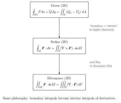
A high-level map of the three major theorems.

9.5.3 Final Practice Problems

Exercise 9.24. Let $C$ be the positively oriented boundary of the region $D=\{(x,y):0\le x\le 1,\ 0\le y\le x\}$. Compute $\displaystyle \oint_C (y^2)\,dx + (x^2)\,dy$ using Green’s theorem.

Exercise 9.25. Let $S$ be the portion of the plane $x+2y+3z=6$ in the first octant, oriented with upward-pointing normal (positive $z$-component). Use Stokes’ theorem to compute $\displaystyle \oint_{\partial S} \langle y,-x,0\rangle\cdot d\boldsymbol{r}$. (Hint: choose a convenient spanning surface with the same boundary.)

Exercise 9.26. Let $S$ be the boundary of the region $E=\{(x,y,z):x^2+y^2+z^2\le 9\}$ oriented outward. Compute $\displaystyle \iint_S \langle x,0,0\rangle\cdot \boldsymbol{n}\,dS$ using the divergence theorem.

Chapter 9 Checklist

Green’s theorem (2D): $\displaystyle \oint_{\partial D} P\,dx+Q\,dy=\iint_D (Q_x-P_y)\,dA$ and flux form $\displaystyle \oint_{\partial D} \boldsymbol{F}\cdot \boldsymbol{n}\,ds=\iint_D (P_x+Q_y)\,dA$.
Stokes’ theorem (3D): $\displaystyle \oint_{\partial S}\boldsymbol{F}\cdot d\boldsymbol{r}=\iint_S (\nabla\times\boldsymbol{F})\cdot \boldsymbol{n}\,dS$.
Divergence theorem (3D): $\displaystyle \iint_{\partial E}\boldsymbol{F}\cdot \boldsymbol{n}\,dS=\iiint_E (\nabla\cdot\boldsymbol{F})\,dV$.
Orientation matters: counterclockwise in the plane, right-hand rule in space, outward for closed surfaces.
Strategy: choose the theorem that converts your integral into the simplest region/surface/volume integral available.

1 Chapter 1: Vectors and the Geometry of Space

1.1 Lesson 1.1: Vectors in Two and Three Dimensions

1.1.1 Scalars and Vectors

1.1.2 Geometric Interpretation and Component Form

1.1.3 Magnitude, Distance, and Unit Vectors

1.1.4 Standard Basis and Direction Cosines

1.2 Lesson 1.2: Vector Operations

1.2.1 Addition, Subtraction, and Scalar Multiplication

1.2.2 Linear Combinations and Span

1.2.3 Basic Vector Identities

1.3 Lesson 1.3: The Dot Product

1.3.1 Definition and Algebraic Properties

1.3.2 Geometric Interpretation, Angles, and Orthogonality

1.3.3 Projections

1.4 Lesson 1.4: The Cross Product

1.4.1 Definition and Computation

1.4.2 Geometry: Orientation and Area

1.5 Lesson 1.5: Lines and Planes in Space

1.5.1 Vector and Parametric Equations of Lines

1.5.2 Equations of Planes

1.5.3 Distances Between Points, Lines, and Planes

Chapter 1 Checklist

2 Chapter 2: Vector-Valued Functions and Space Curves

2.1 Lesson 2.1: Vector-Valued Functions

2.1.1 Definitions and Examples

2.1.2 Limits and Continuity

2.1.3 Graphs of Vector-Valued Functions (Parametric Curves)

2.2 Lesson 2.2: Derivatives of Vector-Valued Functions

2.2.1 Componentwise Differentiation

2.2.2 Velocity and Acceleration Vectors

2.2.3 Tangent Vectors and Tangent Lines

2.3 Lesson 2.3: Integrals of Vector-Valued Functions

2.3.1 Antiderivatives

2.3.2 Definite Integrals

2.3.3 Applications to Motion

2.4 Lesson 2.4: Arc Length and Curvature

2.4.1 Arc Length of Space Curves

2.4.2 Unit Tangent and Normal Vectors

2.4.3 Curvature of a Curve

2.5 Lesson 2.5: Motion in Space

2.5.1 Kinematics in Three Dimensions

Chapter 2 Checklist

3 Chapter 3: Functions of Several Variables

3.1 Lesson 3.1: Functions of Two and Three Variables

3.1.1 Definitions and Examples

3.1.2 Graphs and Level Sets

3.1.3 Domains and Ranges (Geometric View)

3.2 Lesson 3.2: Limits and Continuity

3.2.1 Limits of Multivariable Functions

3.2.2 When a Limit Does Not Exist

3.2.3 Continuity and Properties

3.3 Lesson 3.3: Partial Derivatives

3.3.1 Definition of Partial Derivatives

3.3.2 Higher-Order Partial Derivatives

3.3.3 Clairaut’s Theorem (Equality of Mixed Partials)

3.4 Lesson 3.4: Differentiability and the Gradient

3.4.1 Differentiability

3.4.2 The Gradient Vector

3.4.3 Directional Derivatives

3.5 Lesson 3.5: The Chain Rule

3.5.1 Chain Rule for One Parameter

3.5.2 Chain Rule for Two Parameters

3.5.3 Implicit Differentiation

Chapter 3 Checklist

4 Chapter 4: Applications of Partial Derivatives

4.1 Lesson 4.1: Tangent Planes and Linear Approximations

4.1.1 Tangent Plane to a Surface \(z=f(x,y)\)

4.1.2 Linearization (Best Local Linear Approximation)

4.1.3 Error Estimates (Second-Order Control)

4.2 Lesson 4.2: Extrema of Functions of Several Variables

4.2.1 Critical Points and Local Extrema

4.2.2 Global Extrema on Closed and Bounded Regions

4.3 Lesson 4.3: The Second Derivative Test

4.3.1 The Hessian Matrix and Quadratic Approximation

4.3.2 Classification in Two Variables

4.4 Lesson 4.4: Constrained Optimization

4.4.1 Lagrange Multipliers: Statement

4.4.2 How to Use Lagrange Multipliers (Algorithm)

4.4.3 Worked Examples

Chapter 4 Checklist