Computing and AI

Causal Inference

English · 284 pp. PDF

Chapter 1. Review of Key Statistical Concepts

Lecture 1.1. Populations, Parameters, Estimators, and Inference

1.1 Target Population

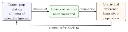
Statistics begins with a scientific question about a population. The population is not merely the data set on the analyst’s computer. It is the collection of units about which we want to learn.

Definition 1.1 (Target population). The target population is the collection of units, real or conceptual, to which the scientific conclusion is intended to apply. A unit might be a person, hospital, county, clinic visit, gene, school, or any other entity on which variables can be defined.

In many applications the target population is partly hypothetical. For example, suppose the scientific goal is to learn the average systolic blood pressure among adults in the United States between ages 65 and 100. We cannot observe every such person in every possible setting in which they might have been sampled. Nevertheless, the target population is the conceptual object that defines what the analysis is trying to describe.

This distinction matters because the same data can be used to answer different population-level questions. A data set from three health systems might be used to learn about patients in those systems, about patients in similar integrated health systems, or about a broader national patient population. These are different targets. The data may be identical, but the scientific claim changes when the population changes.

Key Idea

The data are not the final object of interest. The data are evidence about a population quantity that we cannot observe directly.

A sample is a finite piece of evidence about a larger target population.

1.2 Target Parameter and Estimand

After specifying the population, the next task is to specify the number, function, or distributional feature we want to learn.

Definition 1.2 (Target parameter). A target parameter is a well-defined summary of the target population distribution. It is the quantity the analysis aims to learn. The word estimand is often used synonymously, especially when emphasizing the quantity to be estimated.

Examples include:

the population mean systolic blood pressure, \(\mathbb{E}(W)\);
the population prevalence of HIV infection, \(\mathbb{P}(Y=1)\);
the difference in mean blood pressure between people observed to take statins and people observed not to take statins, \(\mathbb{E}(Y\,\vert\,A=1)-\mathbb{E}(Y\,\vert\,A=0)\);
a regression function such as \(w \mapsto \mathbb{E}(Y\,\vert\,W=w)\).

A parameter is not the same thing as an observed data point. If one patient has systolic blood pressure 135, that is a measurement. The population mean systolic blood pressure is a property of the distribution of blood pressure in the population. It would still be well-defined even before drawing a sample.

Example 1.3 (A descriptive parameter). Let \(W\) denote age and \(Y\) denote systolic blood pressure for members of a target population. The parameter \(\mathbb{E}(Y)\) is the average systolic blood pressure in that population. The parameter \(\mathbb{E}(Y\,\vert\,W\ge 65)\) is the average systolic blood pressure among the subgroup of the population aged at least 65.

At this point in the course, most parameters are descriptive statistical parameters. Later, causal inference will introduce counterfactual parameters such as \(\mathbb{E}\{Y(1)\}-\mathbb{E}\{Y(0)\}\), which describe populations under interventions. The same discipline applies: first define the population, then define the parameter.

1.3 Data as a Sample from a Population

Let \(O\) denote the full observed data record for one unit. In a simple study we may observe \[O=(W,A,Y),\] where \(W\) is a vector of baseline covariates, \(A\) is an exposure or treatment, and \(Y\) is an outcome. A sample of size \(n\) is written \[O_1,\ldots,O_n.\] A common statistical model assumes that these observations are independent and identically distributed: \[O_1,\ldots,O_n \overset{\mathrm{iid}}{\sim}P,\] where \(P\) is the population distribution.

Definition 1.4 (Iid sample). The observations \(O_1,\ldots,O_n\) are independent and identically distributed, written \(O_i \overset{\mathrm{iid}}{\sim}P\), if each observation has the same population distribution \(P\) and the value of one observation does not affect the distribution of another.

The iid assumption is a mathematical idealization. It is reasonable for some sampling schemes and unreasonable for others. For example, measurements from unrelated patients sampled independently from a clinic may be close to iid. Measurements from repeated visits of the same patient are not iid unless the unit is redefined or the dependence is modeled.

The distribution \(P\) determines the target parameter. For instance, if the parameter is the population mean of \(Y\), then \[\psi(P)=\mathbb{E}_P(Y).\] The notation \(\psi(P)\) reminds us that a parameter is a function of the population distribution. If the population distribution changed, the parameter would generally change.

1.4 Point Estimates and Estimators

Because the population distribution \(P\) is unknown, the target parameter \(\psi(P)\) is unknown. Statistical inference uses the sample to construct an estimate.

Definition 1.5 (Estimator and point estimate). An estimator is a rule or algorithm that maps a data set to a numerical estimate of a target parameter. A point estimate is the numerical value produced by the estimator in the observed data.

For example, suppose the target parameter is the population mean \(\psi=\mathbb{E}(Y)\). The sample mean estimator is \[\hat\psi_n=\frac{1}{n}\sum_{i=1}^n Y_i.\] The expression \(\hat\psi_n\) is the estimator as a formula. After observing the actual \(Y_1,\ldots,Y_n\), the resulting number is the point estimate.

Estimation Notes

For the population mean \(\psi=\mathbb{E}(Y)\): \[\text{estimand: } \psi=\mathbb{E}(Y), \qquad \text{estimator: } \hat\psi_n=\frac{1}{n}\sum_{i=1}^n Y_i.\] The estimator is the recipe. The point estimate is the recipe’s output on the observed data.

The distinction between estimand, estimator, and estimate is essential.

The estimand is the population quantity we want.
The estimator is the method used to learn it from data.
The estimate is the number obtained in this particular sample.

1.5 Standard Errors

If the study were repeated on a new random sample from the same population, the estimate would usually change. A standard error describes this repeated-sampling variability.

Definition 1.6 (Standard error). The standard error of an estimator \(\hat\psi_n\) is the standard deviation of its sampling distribution: \[\operatorname{SE}(\hat\psi_n)=\sqrt{\mathop{\mathrm{Var}}(\hat\psi_n)}.\] An estimated standard error is a data-based estimate of this quantity.

For the sample mean under iid sampling with \(\mathop{\mathrm{Var}}(Y)=\sigma^2<\infty\), \[\mathop{\mathrm{Var}}(\hat\psi_n) =\mathop{\mathrm{Var}}\left(\frac{1}{n}\sum_{i=1}^n Y_i\right) =\frac{1}{n^2}\sum_{i=1}^n \mathop{\mathrm{Var}}(Y_i) =\frac{n\sigma^2}{n^2} =\frac{\sigma^2}{n}.\] Thus \[\operatorname{SE}(\hat\psi_n)=\frac{\sigma}{\sqrt n}.\] Since \(\sigma\) is unknown, it is commonly replaced by the sample standard deviation \(s_n\), yielding \[\widehat{\operatorname{SE}}(\hat\psi_n)=\frac{s_n}{\sqrt n}.\]

The standard error is not the same as the standard deviation of \(Y\). The standard deviation of \(Y\) describes variability among individuals in the population. The standard error describes variability of the estimator across repeated samples.

1.6 Confidence Intervals

A point estimate gives one best guess. A confidence interval gives a range of values that accounts for sampling variability.

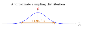
Many estimators used in large samples are approximately Normal: \[\hat\psi_n \approx \operatorname{Normal}\{\psi,\operatorname{SE}(\hat\psi_n)^2\}.\] When an estimator is approximately Normal and its standard error can be estimated, a common Wald-style \(95\%\) confidence interval is \[\hat\psi_n \pm 1.96\,\widehat{\operatorname{SE}}(\hat\psi_n).\]

Definition 1.7 (Frequentist confidence interval). A procedure for constructing \(95\%\) confidence intervals has \(95\%\) coverage if, under repeated sampling from the same population, approximately \(95\%\) of the intervals it produces contain the true target parameter.

The interpretation is about the procedure, not about the fixed realized interval. In frequentist inference the parameter \(\psi\) is treated as fixed. The random object is the interval, because the interval changes from sample to sample.

A Wald interval uses the approximate Normal sampling distribution of the estimator.

1.7 Hypothesis Tests

A hypothesis test turns data into a decision about a proposed value or claim.

Definition 1.8 (Null and alternative hypotheses). A null hypothesis \(H_0\) is a default claim about the target parameter, often representing no difference or no association. An alternative hypothesis \(H_1\) is the claim against which the null is compared.

For example, if \(\psi\) is a difference in population means, a common null hypothesis is \[H_0:\psi=0,\] with a two-sided alternative \[H_1:\psi\ne 0.\] If \(\hat\psi_n\) is approximately Normal, a Wald test statistic is \[Z=\frac{\hat\psi_n-\psi_0}{\widehat{\operatorname{SE}}(\hat\psi_n)},\] where \(\psi_0\) is the value specified by the null hypothesis. Under \(H_0\) and appropriate regularity conditions, \(Z\) is approximately standard Normal. Large values of \(\left\lvert Z\right\rvert\) are evidence against \(H_0\).

The \(p\)-value for a two-sided Wald test is \[p=2\{1-\Phi(\left\lvert Z\right\rvert)\},\] where \(\Phi\) is the standard Normal cumulative distribution function.

Key Idea

Point estimates, standard errors, confidence intervals, and hypothesis tests are all tools for learning about a target parameter. None of them is meaningful until the target population and target parameter have been clearly defined.

Lecture 1.2. Frequentist and Bayesian Perspectives

2.1 Frequentist Interpretation of Probability

In the frequentist view, probabilities describe long-run relative frequencies in a repeatable process or proportions in a target population. If \(A\) is an indicator that a person received a monoclonal antibody infusion and \(Y\) is an indicator of HIV infection, then \[\mathbb{P}(A=1,Y=1)\] can be read as the proportion of the target population for whom both \(A=1\) and \(Y=1\).

This interpretation also applies to conditional probabilities. The probability \[\mathbb{P}(Y=1\,\vert\,A=1)\] is the proportion infected among the subgroup who received monoclonal antibodies. The conditioning event defines the subgroup; the probability describes the fraction of that subgroup with the outcome.

For continuous variables the exact phrase "proportion with \(W=w\)" may be inappropriate because \(\mathbb{P}(W=w)\) can equal zero. In that setting probability is described by densities, distribution functions, and probabilities of intervals such as \(\mathbb{P}(60\le W\le 70)\). The conceptual role is the same: probability describes how values are distributed in a population or under a random experiment.

2.2 Bayesian Updating

The Bayesian view treats unknown quantities as objects about which uncertainty can be expressed probabilistically. A Bayesian analysis begins with a prior distribution, combines it with the likelihood supplied by the data, and obtains a posterior distribution.

Definition 2.1 (Bayesian update). Let \(\theta\) denote an unknown parameter and let \(O_1,\ldots,O_n\) denote observed data. A Bayesian analysis specifies a prior density \(\pi(\theta)\) and a likelihood \(L(\theta;O_1,\ldots,O_n)\). The posterior density is \[\pi(\theta\,\vert\,O_1,\ldots,O_n) = \frac{L(\theta;O_1,\ldots,O_n)\pi(\theta)} {\int L(t;O_1,\ldots,O_n)\pi(t)\,dt}.\]

In words, the posterior distribution is the updated state of uncertainty after seeing the data. The denominator makes the posterior integrate to one. It also shows a central feature of Bayesian inference: prior beliefs and the likelihood both contribute to the final answer.

For example, if \(\theta\) is the prevalence of a disease, a Bayesian credible interval might be interpreted as an interval containing \(\theta\) with posterior probability \(0.95\), conditional on the model and prior. This differs from a frequentist confidence interval, whose \(95\%\) statement concerns repeated-sampling coverage of the interval construction procedure.

2.3 Repeated-Sampling Properties

Frequentist inference evaluates statistical procedures by imagining repeated samples from the same population. If the study were repeated many times, each repetition would produce a new data set, a new point estimate, a new confidence interval, and perhaps a new hypothesis test decision.

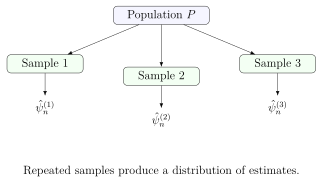
Frequentist properties describe how a procedure behaves over repeated samples.

The phrase "good procedure" means that the procedure reliably achieves its stated goal over these repetitions. A good estimator is close to the truth on average or in large samples. A good confidence interval procedure contains the true parameter at its advertised rate. A good test rejects false null hypotheses often while controlling false rejection under the null.

2.4 Bias

Definition 2.2 (Bias). The finite-sample bias of an estimator \(\hat\psi_n\) for a parameter \(\psi\) is \[\mathop{\mathrm{Bias}}(\hat\psi_n)=\mathbb{E}(\hat\psi_n)-\psi,\] where the expectation is taken over repeated samples from the population.

Bias is an average error across repeated experiments. It is not the error in one realized data set. An estimator can be biased and still sometimes be close to the truth; it can also be unbiased and still be highly variable.

Example 2.3 (Bias of the sample mean). If \(Y_1,\ldots,Y_n \overset{\mathrm{iid}}{\sim}P\) and \(\psi=\mathbb{E}(Y)\), then the sample mean is unbiased: \[\mathbb{E}(\hat\psi_n) =\mathbb{E}\left(\frac{1}{n}\sum_{i=1}^nY_i\right) =\frac{1}{n}\sum_{i=1}^n\mathbb{E}(Y_i) =\frac{1}{n}\sum_{i=1}^n\psi =\psi.\] Therefore \(\mathop{\mathrm{Bias}}(\hat\psi_n)=0\).

Large-sample theory often focuses on whether the bias disappears as \(n\) grows. An estimator is consistent if it converges in probability to the truth: \[\hat\psi_n \overset{P}{\longrightarrow} \psi.\] Consistency is stronger than saying the estimator is approximately unbiased in large samples, because it also requires the estimator’s variability to vanish.

2.5 Sampling Distribution

Definition 2.4 (Sampling distribution). The sampling distribution of an estimator is the probability distribution of the estimator over repeated samples from the same population.

The sampling distribution answers the question: if we repeatedly collected samples of size \(n\) and computed the same estimator each time, what values would the estimator take and how often?

For the sample mean, the central limit theorem gives an approximate answer. If \(Y_1,\ldots,Y_n\) are iid with mean \(\psi\) and variance \(\sigma^2<\infty\), then \[\frac{\hat\psi_n-\psi}{\sigma/\sqrt n} \overset{d}{\longrightarrow} \operatorname{Normal}(0,1).\] Equivalently, for large \(n\), \[\hat\psi_n \approx \operatorname{Normal}\left(\psi,\frac{\sigma^2}{n}\right).\] This approximation is the basis for many standard errors, confidence intervals, and Wald tests.

2.6 Coverage Probability

Suppose an interval procedure maps each data set to an interval \(C_n\). For example, \[C_n=\left[ \hat\psi_n-1.96\,\widehat{\operatorname{SE}}(\hat\psi_n), \hat\psi_n+1.96\,\widehat{\operatorname{SE}}(\hat\psi_n) \right].\]

Definition 2.5 (Coverage probability). The coverage probability of an interval procedure \(C_n\) is \[\mathbb{P}\{\psi\in C_n\},\] where the probability is over repeated samples. A nominal \(95\%\) confidence interval procedure aims to have coverage probability close to \(0.95\).

Coverage is a property of the procedure, not a property of the one interval obtained in the observed data. Once a particular interval has been computed, it either contains the fixed parameter or it does not. The frequentist probability statement refers to what would happen if the entire data-generating process were repeated.

2.7 Power

Hypothesis testing has its own repeated-sampling properties. Consider a test of \[H_0:\psi=\psi_0\] against some alternative. A test is a rule that rejects or fails to reject \(H_0\).

Definition 2.6 (Type I error and power). The Type I error rate is the probability of rejecting \(H_0\) when \(H_0\) is true. The power of a test at a particular alternative value \(\psi\ne\psi_0\) is the probability of rejecting \(H_0\) when that alternative is true.

Power depends on the true effect size, the sample size, the variability of the estimator, and the rejection threshold. Larger sample sizes often increase power because they reduce standard errors, making it easier to distinguish a real difference from sampling noise.

Key Idea

Frequentist and Bayesian analyses answer uncertainty questions differently. Frequentist statements evaluate procedures under repeated sampling. Bayesian statements update probability distributions for unknown quantities conditional on a prior, likelihood, and observed data.

Lecture 1.3. Probability Foundations

3.1 Joint Distributions

Probability distributions describe how variables vary in a population. When more than one variable is considered at the same time, the relevant object is a joint distribution.

Definition 3.1 (Joint distribution). For discrete variables \(X\) and \(Y\), the joint distribution assigns probabilities \[\mathbb{P}(X=x,Y=y)\] to every possible pair of values \((x,y)\). For continuous variables, the joint distribution is described by a joint density or by probabilities of regions.

The joint distribution contains information about each variable separately and about how the variables relate to each other. If \(A\) denotes monoclonal antibody receipt and \(Y\) denotes HIV infection status, then \[\mathbb{P}(A=1,Y=1)\] is the proportion of the target population who both received monoclonal antibodies and are HIV infected.

If \(W\) denotes age, then \[\mathbb{P}(W=65,A=1,Y=0)\] is the proportion of the population who are exactly 65 years old, received monoclonal antibodies, and are not HIV infected. For continuous age, one would usually use an interval such as \(\mathbb{P}(65\le W<66,A=1,Y=0)\).

3.2 Marginal Distributions

A marginal distribution describes one variable or a subset of variables without conditioning on the remaining variables.

Definition 3.2 (Marginal distribution). For discrete variables \(X\) and \(Y\), the marginal distribution of \(X\) is obtained from the joint distribution by summing over all possible values of \(Y\): \[\mathbb{P}(X=x)=\sum_y \mathbb{P}(X=x,Y=y).\]

This operation is called marginalization. It removes a variable by adding over its possible values.

Example 3.3 (Marginalizing over treatment). Let \(Y\) be HIV infection status and \(A\) be monoclonal antibody receipt. The population prevalence of HIV infection is \[\mathbb{P}(Y=1) =\mathbb{P}(Y=1,A=0)+\mathbb{P}(Y=1,A=1) =\sum_{a=0}^1 \mathbb{P}(Y=1,A=a).\] The total infected group is partitioned into infected nonrecipients and infected recipients.

A marginal probability is obtained by adding joint probabilities over the variables being removed.

3.3 Conditional Distributions

Conditional probability describes a distribution inside a subgroup.

Definition 3.4 (Conditional distribution). For discrete variables \(X\) and \(Y\) with \(\mathbb{P}(Y=y)>0\), \[\mathbb{P}(X=x\,\vert\,Y=y) = \frac{\mathbb{P}(X=x,Y=y)}{\mathbb{P}(Y=y)}.\]

The denominator restricts attention to the subgroup with \(Y=y\). The numerator counts the part of that subgroup that also has \(X=x\). Thus conditional probability is a subgroup proportion.

Example 3.5 (HIV infection among monoclonal recipients). The probability of HIV infection among monoclonal antibody recipients is \[\mathbb{P}(Y=1\,\vert\,A=1) = \frac{\mathbb{P}(Y=1,A=1)}{\mathbb{P}(A=1)}.\] This is not the fraction infected in the whole population. It is the fraction infected among the recipient subgroup.

With covariates, conditioning can define very specific subgroups. If \(W=(W_1,W_2,W_3)\) represents age, BMI, and profession, then \(W=w=(65,28.5,\text{nurse})\) defines the subgroup of 65-year-old nurses with BMI 28.5. A probability such as \[\mathbb{P}(Y=1\,\vert\,A=1,W=w)\] is the probability of infection among monoclonal recipients in that covariate-defined subgroup.

3.4 Chain Rule Factorization

The definition of conditional probability can be rearranged to express a joint distribution as a product.

Proposition 3.6 (Chain rule for two variables). If \(\mathbb{P}(X=x)>0\) and \(\mathbb{P}(Y=y)>0\), then \[\mathbb{P}(X=x,Y=y) =\mathbb{P}(X=x)\mathbb{P}(Y=y\,\vert\,X=x) =\mathbb{P}(Y=y)\mathbb{P}(X=x\,\vert\,Y=y).\]

Proof. By the definition of conditional probability, \[\mathbb{P}(Y=y\,\vert\,X=x) =\frac{\mathbb{P}(X=x,Y=y)}{\mathbb{P}(X=x)}.\] Multiplying both sides by \(\mathbb{P}(X=x)\) gives \[\mathbb{P}(X=x)\mathbb{P}(Y=y\,\vert\,X=x)=\mathbb{P}(X=x,Y=y).\] The second factorization follows by the same argument with \(X\) and \(Y\) interchanged. ◻

For three variables, repeated application gives \[\mathbb{P}(W=w,A=a,Y=y) = \mathbb{P}(W=w)\mathbb{P}(A=a\,\vert\,W=w)\mathbb{P}(Y=y\,\vert\,A=a,W=w).\] This factorization is a purely probabilistic identity. It does not by itself imply any causal ordering.

3.5 Bayes Rule

Bayes rule follows by combining the two chain rule factorizations.

Proposition 3.7 (Bayes rule). If \(\mathbb{P}(Y=y)>0\), then \[\mathbb{P}(X=x\,\vert\,Y=y) = \frac{\mathbb{P}(Y=y\,\vert\,X=x)\mathbb{P}(X=x)}{\mathbb{P}(Y=y)}.\] Moreover, \[\mathbb{P}(Y=y)=\sum_x \mathbb{P}(Y=y\,\vert\,X=x)\mathbb{P}(X=x)\] in the discrete case.

Proof. The chain rule gives \[\mathbb{P}(X=x,Y=y)=\mathbb{P}(Y=y\,\vert\,X=x)\mathbb{P}(X=x).\] Substitute this expression into the definition \[\mathbb{P}(X=x\,\vert\,Y=y)=\frac{\mathbb{P}(X=x,Y=y)}{\mathbb{P}(Y=y)}\] to obtain Bayes rule. The expression for \(\mathbb{P}(Y=y)\) follows by marginalizing over \(X\) and then applying the chain rule: \[\mathbb{P}(Y=y) =\sum_x\mathbb{P}(X=x,Y=y) =\sum_x\mathbb{P}(Y=y\,\vert\,X=x)\mathbb{P}(X=x).\] ◻

3.6 From Joint to Marginal Probabilities

The operation from joint to marginal probabilities is adding or integrating. For discrete variables, \[\mathbb{P}(X=x)=\sum_y \mathbb{P}(X=x,Y=y).\] For continuous variables with joint density \(f_{X,Y}\), \[f_X(x)=\int f_{X,Y}(x,y)\,dy.\] The same principle applies to mixed or higher-dimensional data. For example, \[\mathbb{P}(W=25,A=1) = \sum_{y=0}^1 \mathbb{P}(W=25,A=1,Y=y),\] and \[\mathbb{P}(W=25) = \sum_{a=0}^1\sum_{y=0}^1 \mathbb{P}(W=25,A=a,Y=y).\]

The idea is simple: to ignore a variable, add over every way that variable could have occurred.

3.7 Conditional Probability as Subgroup Proportion

The most important intuition in this lecture is that conditioning defines a subgroup.

Key Idea

Conditional probability equals a proportion within a subgroup: \[\mathbb{P}(\text{characteristic}\,\vert\,\text{subgroup}) = \frac{\mathbb{P}(\text{characteristic and subgroup})} {\mathbb{P}(\text{subgroup})}.\]

For instance, \[\mathbb{P}(Y=1\,\vert\,W=25,A=1) = \frac{\mathbb{P}(Y=1,W=25,A=1)}{\mathbb{P}(W=25,A=1)}.\] The denominator is the proportion of the whole population who are 25-year-old monoclonal recipients. The numerator is the proportion of the whole population who are 25-year-old monoclonal recipients and HIV infected. Dividing converts the whole-population proportion into a within-subgroup proportion.

This subgroup interpretation will be used constantly in causal inference. When we later write expressions such as \(\mathbb{E}(Y\,\vert\,A=1,W=w)\) or \(\mathbb{P}(A=1\,\vert\,W=w)\), the conditioning variables define the subgroup in which an outcome mean or treatment probability is being described.

Lecture 1.4. Independence and Conditional Independence

4.1 Definition of Independence

Independence formalizes the idea that learning one piece of information does not change what we know about another.

Definition 4.1 (Independence). Events \(B\) and \(C\) are independent if \[\mathbb{P}(B,C)=\mathbb{P}(B)\mathbb{P}(C).\] Equivalently, when \(\mathbb{P}(C)>0\) and \(\mathbb{P}(B)>0\), \[\mathbb{P}(B\,\vert\,C)=\mathbb{P}(B) \qquad\text{and}\qquad \mathbb{P}(C\,\vert\,B)=\mathbb{P}(C).\] For random variables \(X\) and \(Y\), we write \(X\perp\!\!\!\perp Y\) if all events determined by \(X\) are independent of all events determined by \(Y\).

The equivalence follows directly from conditional probability. If \(\mathbb{P}(B,C)=\mathbb{P}(B)\mathbb{P}(C)\), then \[\mathbb{P}(B\,\vert\,C)=\frac{\mathbb{P}(B,C)}{\mathbb{P}(C)} =\frac{\mathbb{P}(B)\mathbb{P}(C)}{\mathbb{P}(C)} =\mathbb{P}(B).\] Thus conditioning on \(C\) does not change the probability of \(B\).

Key Idea

Independence means that one variable carries no information about the other in the population.

4.2 Definition of Conditional Independence

Conditional independence is independence within strata of another variable.

Definition 4.2 (Conditional independence). Events \(B\) and \(C\) are conditionally independent given \(D\) if \[\mathbb{P}(B,C\,\vert\,D)=\mathbb{P}(B\,\vert\,D)\mathbb{P}(C\,\vert\,D)\] whenever the conditioning probabilities are well-defined. Equivalently, \[\mathbb{P}(B\,\vert\,C,D)=\mathbb{P}(B\,\vert\,D).\] For random variables, we write \(X\perp\!\!\!\perp Y\,\vert\,Z\).

Plainly, \(X\perp\!\!\!\perp Y\,\vert\,Z\) means that after restricting to people with the same value of \(Z\), knowing \(Y\) gives no additional information about \(X\).

Conditional independence is not the same as marginal independence. It is possible for two variables to be associated in the full population but independent within strata of a third variable. It is also possible for two variables to be independent in the full population but associated after conditioning.

4.3 Independence in Randomized Trials

Consider a randomized trial in which \(A\) indicates assignment to a vaccine arm, with \[\mathbb{P}(A=1)=\frac{1}{2}\] for every participant. Let \(W\) denote age. Because the treatment assignment is generated by a random device that ignores age, \[\mathbb{P}(A=1\,\vert\,W=w)=\mathbb{P}(A=1)=\frac{1}{2}\] for every age \(w\) in the trial population. Hence \(A\perp\!\!\!\perp W\).

Causal Assumption

In an individually randomized trial with equal allocation, treatment assignment is independent of baseline covariates: \[A\perp\!\!\!\perp W.\] In plain language, baseline characteristics do not help predict treatment assignment because the randomization mechanism did not use them.

This independence is a design property. It is not discovered by observing that the treatment groups look similar in one finite sample. In a small randomized trial the realized treatment group may contain older participants by chance, but the assignment mechanism is still independent of age.

4.4 Stratified Randomization

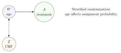
Now suppose the trial uses stratified randomization by age. Participants younger than 65 receive vaccine with probability \(1/2\), while participants aged at least 65 receive vaccine with probability \(2/3\): \[\mathbb{P}(A=1\,\vert\,W<65)=\frac{1}{2}, \qquad \mathbb{P}(A=1\,\vert\,W\ge 65)=\frac{2}{3}.\] In this design, \(A\) and \(W\) are not marginally independent. Knowing that someone is at least 65 changes the probability of treatment assignment.

However, within age strata, the assignment may still be randomized with respect to other baseline covariates. Let \(Z\) denote congestive heart failure status. If the randomization rule uses age but not \(Z\), then \[A\perp\!\!\!\perp Z\,\vert\,W.\] Among people of the same age stratum, knowing congestive heart failure status gives no additional information about treatment assignment.

In a stratified trial, treatment assignment can depend on the stratifying variable while remaining independent of other covariates within strata.

4.5 Why Conditioning Can Remove Information

Conditioning can remove information because it compares units only within a fixed subgroup. In the stratified randomization example, congestive heart failure status may be associated with age. In the full population, learning \(Z\) tells us something about likely age, and age tells us something about treatment probability. Therefore \(Z\) can be informative about \(A\) marginally.

Once we condition on age, that indirect information path is removed. Among participants in the same age stratum, \(Z\) no longer conveys information about the randomization probability. This is why \[A\not\!\perp\!\!\!\perp Z \qquad\text{but}\qquad A\perp\!\!\!\perp Z\,\vert\,W\] can both be true.

The following table gives a concrete illustration: \[\begin{array}{c|cc} & \mathbb{P}(A=1\,\vert\,W,Z=0) & \mathbb{P}(A=1\,\vert\,W,Z=1)\\ \hline W<65 & 1/2 & 1/2\\ W\ge 65 & 2/3 & 2/3 \end{array}\] Within each age stratum, the treatment probability does not depend on \(Z\). If people with \(Z=1\) are more often in the older stratum, then \(\mathbb{P}(A=1\,\vert\,Z=1)\) can still exceed \(\mathbb{P}(A=1\,\vert\,Z=0)\) marginally.

4.6 Why Conditional Independence Matters for Causal Inference

Causal inference often requires comparing treated and untreated people who are similar with respect to variables that affect treatment and outcome. The mathematical language for this idea is conditional independence.

In later chapters, a central causal assumption for a binary treatment will take the form \[Y(a)\perp\!\!\!\perp A\,\vert\,W, \qquad a\in\{0,1\}.\] This says that, among people with the same covariates \(W\), treatment assignment \(A\) carries no additional information about the counterfactual outcome under treatment level \(a\). This is a causal version of "as-if randomized within strata of \(W\)."

The probability concepts in this lecture are therefore not merely technical preliminaries. They are the language used to state whether observed data can support causal comparisons.

Key Idea

Marginal independence asks whether two variables are unrelated in the whole population. Conditional independence asks whether they are unrelated after comparing only units in the same stratum of the conditioning variables.

Lecture 1.5. Expectation and Conditional Expectation

5.1 Expected Value

The expected value is the population average of a random variable.

Definition 5.1 (Expected value). For a discrete random variable \(W\), the expected value, expectation, or mean is \[\mathbb{E}(W)=\sum_w w\,\mathbb{P}(W=w),\] where the sum is over all possible values of \(W\). For a continuous random variable with density \(f_W\), the expected value is \[\mathbb{E}(W)=\int w f_W(w)\,dw,\] provided the integral is well-defined.

The discrete formula says: multiply each possible value by the proportion of the population with that value, then add across values. If \(W\) is age, \(\mathbb{E}(W)\) is the average age in the target population. If \(W\) is systolic blood pressure, \(\mathbb{E}(W)\) is the population mean systolic blood pressure.

5.2 Expectation of Transformations

Expectations can also be taken after transforming variables.

Definition 5.2 (Expectation of a transformation). For a function \(f\), the expectation of \(f(W)\) is \[\mathbb{E}\{f(W)\}=\sum_w f(w)\mathbb{P}(W=w)\] in the discrete case, or \[\mathbb{E}\{f(W)\}=\int f(w)f_W(w)\,dw\] in the continuous case.

Examples include: \[\mathbb{E}(W^2), \qquad \mathbb{E}\{\log(W)\}, \qquad \mathbb{E}\{\mathbb{1}(W\ge 65)\}.\] The last example is especially important because indicator functions convert events into numerical variables.

5.3 Binary Variables and Probabilities

If \(Y\) is binary, with possible values 0 and 1, then its expectation equals the probability that it is 1: \[\mathbb{E}(Y) =\sum_{y=0}^1 y\mathbb{P}(Y=y) =0\cdot \mathbb{P}(Y=0)+1\cdot \mathbb{P}(Y=1) =\mathbb{P}(Y=1).\] More generally, for any event \(B\), \[\mathbb{E}\{\mathbb{1}(B)\}=\mathbb{P}(B).\]

Key Idea

Means and probabilities are not separate ideas for binary variables. The mean of a 0/1 variable is the proportion of the population with value 1.

This fact is used constantly. If \(Y\) is a disease indicator, then \(\mathbb{E}(Y)\) is disease prevalence. If \(A\) is a treatment indicator, then \(\mathbb{E}(A)\) is the proportion treated.

5.4 Conditional Expectation as Subgroup Mean

Conditional expectation is the mean within a subgroup.

Definition 5.3 (Conditional expectation for a discrete conditioning event). For a discrete variable \(W\) and an event \(A=a\) with \(\mathbb{P}(A=a)>0\), \[\mathbb{E}(W\,\vert\,A=a)=\sum_w w\,\mathbb{P}(W=w\,\vert\,A=a).\]

For example, if \(W\) is age and \(A=1\) indicates monoclonal antibody receipt, then \[\mathbb{E}(W\,\vert\,A=1)\] is the average age among monoclonal antibody recipients. It is not the average age in the whole population.

If \(Y\) is binary, then \[\mathbb{E}(Y\,\vert\,A=1)=\mathbb{P}(Y=1\,\vert\,A=1).\] Thus the conditional mean of a binary outcome is a conditional probability.

5.5 Conditional Mean as a Function

A conditional mean can be viewed as a function of the conditioning variables. The notation \[\mathbb{E}(W\,\vert\,A)\] does not represent a single number until \(A\) is fixed. It is a random variable whose value depends on the subgroup to which the unit belongs: \[\mathbb{E}(W\,\vert\,A) = \begin{cases} \mathbb{E}(W\,\vert\,A=0), & A=0,\\ \mathbb{E}(W\,\vert\,A=1), & A=1. \end{cases}\]

In contrast, \(\mathbb{E}(W\,\vert\,A=a)\) is a number once \(a\) is specified.

A conditional expectation can be understood as a function that maps subgroup labels to subgroup means.

5.6 Interpreting \(\mathbb{E}(Y\,\vert\,A,W)\)

The expression \(\mathbb{E}(Y\,\vert\,A,W)\) is a conditional mean function of both treatment and covariates. If \(A\) is binary and \(W\) is age, then \[(a,w)\mapsto \mathbb{E}(Y\,\vert\,A=a,W=w)\] maps each treatment-age subgroup to the mean outcome in that subgroup.

If \(Y\) is binary, then \[\mathbb{E}(Y\,\vert\,A=a,W=w)=\mathbb{P}(Y=1\,\vert\,A=a,W=w).\] For instance, \[\mathbb{E}(Y\,\vert\,A=1,W=65)\] is the outcome prevalence among treated 65-year-olds. It should not be interpreted as the outcome that would occur if a particular person were treated. It is a descriptive mean among people actually observed with \(A=1\) and \(W=65\).

Remark 27. The expression \(\mathbb{E}(Y\,\vert\,A,W)\) is often estimated by regression. A fitted regression model is therefore best understood as an estimated conditional mean function. This interpretation is more fundamental for this course than interpreting individual regression coefficients.

Lecture 1.6. The Tower Rule

6.1 Plain-Language Statement of the Tower Rule

The tower rule is one of the most useful identities in probability and statistics. It says that an overall mean can be recovered by averaging subgroup means, using the subgroup sizes as weights.

Key Idea

The marginal mean equals the average of conditional means, weighted by subgroup prevalence.

Suppose \(W\) is systolic blood pressure and \(A\) is sex at birth, coded as \(A=0\) for one group and \(A=1\) for another. Every person belongs to exactly one subgroup defined by \(A\). If we know the mean blood pressure in each subgroup and the fraction of the population in each subgroup, then we can reconstruct the overall population mean.

In words: \[\text{overall mean} = \sum_{\text{subgroups}} (\text{mean within subgroup})(\text{fraction in subgroup}).\]

6.2 Weighted Averages of Subgroup Means

For a discrete grouping variable \(A\), the tower rule is \[\mathbb{E}(W)=\sum_a \mathbb{E}(W\,\vert\,A=a)\mathbb{P}(A=a).\] The weights \(\mathbb{P}(A=a)\) must add to one. The quantities \(\mathbb{E}(W\,\vert\,A=a)\) are subgroup-specific means. The formula is therefore a weighted average of subgroup means.

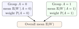
The tower rule combines subgroup means according to subgroup prevalence.

The rule is not an approximation. It is an identity, provided the expectations exist.

6.3 Numeric Example

Suppose the population is split into two groups: \[\mathbb{P}(A=0)=0.6,\qquad \mathbb{P}(A=1)=0.4.\] Suppose the subgroup means of systolic blood pressure are \[\mathbb{E}(W\,\vert\,A=0)=120, \qquad \mathbb{E}(W\,\vert\,A=1)=130.\] Then \[\mathbb{E}(W) =\mathbb{E}(W\,\vert\,A=0)\mathbb{P}(A=0) +\mathbb{E}(W\,\vert\,A=1)\mathbb{P}(A=1).\] Substituting the numbers, \[\mathbb{E}(W) =120(0.6)+130(0.4) =72+52 =124.\] The overall mean is 124. The group representing \(60\%\) of the population contributes \(60\%\) of its mean, and the group representing \(40\%\) contributes \(40\%\) of its mean.

6.4 Probability Notation

The same idea can be written compactly. For discrete \(A\), \[\mathbb{E}(W)=\sum_a \mathbb{E}(W\,\vert\,A=a)\mathbb{P}(A=a).\] For continuous \(A\), the sum is replaced by an integral: \[\mathbb{E}(W)=\int \mathbb{E}(W\,\vert\,A=a) f_A(a)\,da,\] where \(f_A\) is the density of \(A\).

When \(A\) has three values, say \(0,1,2\), the formula is \[\mathbb{E}(W) = \mathbb{E}(W\,\vert\,A=0)\mathbb{P}(A=0) +\mathbb{E}(W\,\vert\,A=1)\mathbb{P}(A=1) +\mathbb{E}(W\,\vert\,A=2)\mathbb{P}(A=2).\]

6.5 Shorthand Form: \(\mathbb{E}(W)=\mathbb{E}\{\mathbb{E}(W\,\vert\,A)\}\)

The tower rule is often written as \[\mathbb{E}(W)=\mathbb{E}\{\mathbb{E}(W\,\vert\,A)\}.\] This notation has two layers:

The inner expression \(\mathbb{E}(W\,\vert\,A)\) is a function of \(A\). It assigns each subgroup its subgroup mean.
The outer expectation averages that function over the population distribution of \(A\).

For binary \(A\), \[\mathbb{E}(W\,\vert\,A) = \begin{cases} \mathbb{E}(W\,\vert\,A=0), & A=0,\\ \mathbb{E}(W\,\vert\,A=1), & A=1. \end{cases}\] Therefore \[\mathbb{E}\{\mathbb{E}(W\,\vert\,A)\} = \mathbb{E}(W\,\vert\,A=0)\mathbb{P}(A=0) +\mathbb{E}(W\,\vert\,A=1)\mathbb{P}(A=1).\]

6.6 Common Mistakes

A common mistake is to confuse \(\mathbb{E}(W\,\vert\,A)\) with \(\mathbb{E}(W)\). The conditional mean \(\mathbb{E}(W\,\vert\,A)\) is generally a random variable because it depends on \(A\). The marginal mean \(\mathbb{E}(W)\) is a single number.

Another common mistake is to omit the subgroup weights. If the subgroup means are 120 and 130, the overall mean is not necessarily \((120+130)/2\). That unweighted average is correct only if the two subgroups are equally prevalent. The correct weights are the population proportions \(\mathbb{P}(A=a)\).

Remark 28. Conditioning creates subgroup-specific quantities. To return to a marginal quantity, we must average over the distribution of the conditioning variable.

6.7 Proof of the Tower Rule

Theorem 6.2 (Tower rule for a discrete grouping variable). Let \(W\) be a discrete random variable with finite expectation and let \(A\) be a discrete random variable. Then \[\mathbb{E}(W)=\sum_a \mathbb{E}(W\,\vert\,A=a)\mathbb{P}(A=a) =\mathbb{E}\{\mathbb{E}(W\,\vert\,A)\}.\]

Proof. Start from the definition of expectation: \[\mathbb{E}(W)=\sum_w w\mathbb{P}(W=w).\] Marginalize over \(A\): \[\mathbb{P}(W=w)=\sum_a \mathbb{P}(W=w,A=a).\] Substitute this into the expectation: \[\mathbb{E}(W) =\sum_w w\sum_a \mathbb{P}(W=w,A=a).\] Switch the order of summation: \[\mathbb{E}(W) =\sum_a\sum_w w\mathbb{P}(W=w,A=a).\] Use the chain rule \(\mathbb{P}(W=w,A=a)=\mathbb{P}(W=w\,\vert\,A=a)\mathbb{P}(A=a)\): \[\mathbb{E}(W) =\sum_a\sum_w w\mathbb{P}(W=w\,\vert\,A=a)\mathbb{P}(A=a).\] Because \(\mathbb{P}(A=a)\) does not depend on \(w\), move it outside the inner sum: \[\mathbb{E}(W) =\sum_a \mathbb{P}(A=a)\sum_w w\mathbb{P}(W=w\,\vert\,A=a).\] The inner sum is the conditional expectation \(\mathbb{E}(W\,\vert\,A=a)\), so \[\mathbb{E}(W)=\sum_a \mathbb{E}(W\,\vert\,A=a)\mathbb{P}(A=a).\] The final expression is exactly \(\mathbb{E}\{\mathbb{E}(W\,\vert\,A)\}\). ◻

6.8 Practice Problems

Exercise 6.3 (Three groups). Let \(A\in\{0,1,2\}\) with \[\mathbb{P}(A=0)=0.2,\qquad \mathbb{P}(A=1)=0.5,\qquad \mathbb{P}(A=2)=0.3.\] Suppose \[\mathbb{E}(W\,\vert\,A=0)=9,\qquad \mathbb{E}(W\,\vert\,A=1)=10,\qquad \mathbb{E}(W\,\vert\,A=2)=14.\] Compute \(\mathbb{E}(W)\).

Solution. Apply the tower rule: \[\mathbb{E}(W) =9(0.2)+10(0.5)+14(0.3) =1.8+5+4.2 =11.\] ◻

Exercise 6.4 (Conditioning on two variables). Let \(A\) and \(Z\) be discrete. Express \(\mathbb{E}(W)\) using subgroup means defined by both \(A\) and \(Z\).

Solution. The joint groups are defined by pairs \((a,z)\). The tower rule gives \[\mathbb{E}(W) = \sum_a\sum_z \mathbb{E}(W\,\vert\,A=a,Z=z)\mathbb{P}(A=a,Z=z).\] Equivalently, \[\mathbb{E}(W)=\mathbb{E}\{\mathbb{E}(W\,\vert\,A,Z)\}.\] ◻

Exercise 6.5 (A conditional version). Let \(A\) and \(Z\) be discrete. Express \(\mathbb{E}(W\,\vert\,A=1)\) using subgroup means defined by \(Z\) among those with \(A=1\).

Solution. Within the subgroup \(A=1\), average over the distribution of \(Z\) in that subgroup: \[\mathbb{E}(W\,\vert\,A=1) = \sum_z \mathbb{E}(W\,\vert\,A=1,Z=z)\mathbb{P}(Z=z\,\vert\,A=1).\] This is the tower rule applied inside the \(A=1\) subpopulation. ◻

Lecture 1.7. Regression as Conditional Expectation Estimation

7.1 Regression as Estimation of \(\mathbb{E}(Y\,\vert\,A,W)\)

In this course, regression will be used primarily as a tool for estimating conditional expectations. This is broader than the common habit of treating regression coefficients as the main scientific output.

Definition 7.1 (Regression function). For outcome \(Y\), treatment or exposure \(A\), and covariates \(W\), the regression function is the conditional mean \[\overline{Q}(a,w)=\mathbb{E}(Y\,\vert\,A=a,W=w).\] An estimator of this function will be denoted \(\hat Q_n(a,w)\) or \(\overline{Q}_n(a,w)\).

The regression function is a machine: input a subgroup specification \((a,w)\), output the mean of \(Y\) among units in that subgroup.

Estimation Notes

Regression workflow for estimating \(\mathbb{E}(Y\,\vert\,A,W)\):

Choose a regression method and a set of predictors involving \(A\) and \(W\).
Fit the regression using the observed data \((Y_i,A_i,W_i)\).
Obtain an estimated function \(\overline{Q}_n(a,w)\).
Evaluate \(\overline{Q}_n(a,w)\) at covariate and treatment values of scientific interest.

7.2 Linear Regression

A main-terms linear regression model for a scalar covariate \(W\) is \[\mathbb{E}(Y\,\vert\,A,W)=\beta_0+\beta_1A+\beta_2W.\] After fitting the model, the estimated regression function is \[\overline{Q}_n(a,w)=\hat\beta_0+\hat\beta_1a+\hat\beta_2w.\]

For example, if the fitted coefficients are \[\hat\beta_0=3.27,\qquad \hat\beta_1=0.17,\qquad \hat\beta_2=-0.18,\] then \[\overline{Q}_n(a,w)=3.27+0.17a-0.18w.\] The estimated mean outcome for untreated people in age group 4 is \[\overline{Q}_n(0,4)=3.27+0.17(0)-0.18(4)=2.55.\] The estimated mean outcome for treated people in age group 7 is \[\overline{Q}_n(1,7)=3.27+0.17(1)-0.18(7)=2.18.\]

The coefficient \(\hat\beta_1\) is the modeled difference between treatment groups holding \(W\) fixed by one unit of the model. Whether that coefficient is itself a meaningful scientific estimand depends on the question and on the model. The safer general view is that the fitted model estimates a conditional mean function.

7.3 Logistic Regression

When the outcome is binary, a conditional mean must lie between 0 and 1. Logistic regression ensures this by modeling the log-odds and then transforming back to a probability.

Definition 7.2 (Expit function). The expit function is \[\mathop{\mathrm{expit}}(x)=\frac{\exp(x)}{1+\exp(x)} =\frac{1}{1+\exp(-x)}.\] It maps every real number to a value in \((0,1)\).

A main-terms logistic regression model is \[\mathbb{E}(Y\,\vert\,A,W) =\mathbb{P}(Y=1\,\vert\,A,W) =\mathop{\mathrm{expit}}(\gamma_0+\gamma_1A+\gamma_2W).\] After fitting, \[\overline{Q}_n(a,w)=\mathop{\mathrm{expit}}(\hat\gamma_0+\hat\gamma_1a+\hat\gamma_2w).\]

If logistic regression is used to estimate the treatment mechanism rather than the outcome regression, one might write \[g(w)=\mathbb{P}(A=1\,\vert\,W=w) =\mathop{\mathrm{expit}}(\alpha_0+\alpha_1w),\] with fitted estimator \[g_n(w)=\mathop{\mathrm{expit}}(\hat\alpha_0+\hat\alpha_1w).\] For example, if \(\hat\alpha_0=-0.44\) and \(\hat\alpha_1=0.07\), then \[g_n(2)=\mathop{\mathrm{expit}}(-0.44+0.07\cdot 2)\approx 0.43,\] and \[g_n(5)=\mathop{\mathrm{expit}}(-0.44+0.07\cdot 5)\approx 0.48.\]

7.4 Generalized Linear Models

Linear and logistic regression are examples of generalized linear models (GLMs). A GLM specifies a conditional mean through a link function: \[h\{\mathbb{E}(Y\,\vert\,X)\}=\eta(X),\] where \(X\) denotes predictors, \(h\) is the link function, and \(\eta(X)\) is a linear predictor.

For linear regression, \(h(u)=u\), so \[\mathbb{E}(Y\,\vert\,X)=\eta(X).\] For logistic regression, \(h(u)=\mathop{\mathrm{logit}}(u)\), so \[\mathop{\mathrm{logit}}\{\mathbb{E}(Y\,\vert\,X)\}=\eta(X), \qquad \mathbb{E}(Y\,\vert\,X)=\mathop{\mathrm{expit}}\{\eta(X)\}.\]

In causal inference applications, GLMs are often used as nuisance regressions: intermediate models needed to estimate a target causal parameter. The final target is often not a regression coefficient.

7.5 Main-Terms Models

A main-terms model includes predictors additively on the scale of the linear predictor. With scalar \(W\), \[\eta(A,W)=\beta_0+\beta_1A+\beta_2W.\] For several covariates \(W=(W_1,\ldots,W_p)\), \[\eta(A,W)=\beta_0+\beta_1A+\beta_2W_1+\cdots+\beta_{p+1}W_p.\]

Main-terms models borrow information across subgroups by imposing a simple structure. In the linear model above, the difference between \(A=1\) and \(A=0\) is the same at every value of \(W\): \[\overline{Q}_n(1,w)-\overline{Q}_n(0,w)=\hat\beta_1.\] That restriction can be useful when data are limited, but it can be wrong if treatment-outcome associations vary across covariate values.

7.6 Interaction Models

Interaction models allow the relationship between one predictor and the outcome to depend on another predictor. A linear model with an \(A\) by \(W\) interaction is \[\mathbb{E}(Y\,\vert\,A,W)=\beta_0+\beta_1A+\beta_2W+\beta_3AW.\] The fitted function is \[\overline{Q}_n(a,w)=\hat\beta_0+\hat\beta_1a+\hat\beta_2w+\hat\beta_3aw.\] Now the fitted difference between treatment groups at covariate value \(w\) is \[\overline{Q}_n(1,w)-\overline{Q}_n(0,w)=\hat\beta_1+\hat\beta_3w.\] Thus the treatment contrast on the outcome scale is allowed to vary with \(W\).

Polynomial terms are another way to add flexibility: \[\eta(A,W)=\beta_0+\beta_1A+\beta_2W+\beta_3W^2.\] The choice of regression formula determines what patterns can and cannot be represented by the fitted conditional mean.

7.7 Using `glm` in R

The R function glm fits generalized linear models. Suppose a data frame covid19 contains:

out: an outcome variable \(Y\);
treat: a binary treatment variable \(A\);
age_grp: an age group covariate \(W\).

A main-terms linear regression for \(\mathbb{E}(Y\,\vert\,A,W)\) is fit by:

fit1 <- glm(out ~ treat + age_grp, data = covid19)
coef(fit1)

If the coefficient output is approximately

(Intercept)      treat    age_grp
     3.2714     0.1692    -0.1780

then the fitted conditional mean is \[\overline{Q}_n(a,w)=3.2714+0.1692a-0.1780w.\]

A main-terms logistic regression for the treatment probability \(\mathbb{P}(A=1\,\vert\,W)\) is fit by:

fit2 <- glm(treat ~ age_grp, data = covid19, family = binomial())
coef(fit2)

If the fitted coefficients are approximately \(-0.4391\) for the intercept and \(0.0729\) for age_grp, then \[g_n(w)=\mathop{\mathrm{expit}}(-0.4391+0.0729w).\]

7.8 Prediction with `newdata`

After fitting a regression, predict evaluates the fitted conditional mean at specified covariate values. For example:

aw_values <- data.frame(
  treat = c(0, 1),
  age_grp = c(4, 7)
)

predict(fit1, newdata = aw_values, type = "response")

The object aw_values contains two subgroup specifications: \((A=0,W=4)\) and \((A=1,W=7)\). The call to predict returns the fitted means \(\overline{Q}_n(0,4)\) and \(\overline{Q}_n(1,7)\).

For logistic regression, type = "response" returns probabilities rather than log-odds:

w_values <- data.frame(age_grp = c(2, 5))
predict(fit2, newdata = w_values, type = "response")

These are estimates of \(\mathbb{P}(A=1\,\vert\,W=2)\) and \(\mathbb{P}(A=1\,\vert\,W=5)\) under the fitted logistic model.

7.9 Regression Output as Subgroup Mean Estimates

Regression output should be translated back into conditional mean estimates. Coefficients are ingredients for constructing the function \(\overline{Q}_n\) or \(g_n\).

Key Idea

A fitted regression is an estimated function. It takes subgroup-defining variables as input and returns an estimated subgroup mean or subgroup probability.

Sometimes we need a function such as \[w\mapsto \mathbb{E}(Y\,\vert\,A=1,W=w)\] rather than the full function \((a,w)\mapsto \mathbb{E}(Y\,\vert\,A=a,W=w)\). There are two common approaches.

Pooling.

Fit a regression using all observations and include \(A\) and \(W\) as predictors. If \[\overline{Q}_n(a,w)=\hat\beta_0+\hat\beta_1a+\hat\beta_2w,\] then estimate the treated conditional mean by setting \(a=1\): \[\overline{Q}_{n,1}(w)=\overline{Q}_n(1,w)=\hat\beta_0+\hat\beta_1+\hat\beta_2w.\]

Stratifying.

Restrict the data to observations with \(A=1\) and regress \(Y\) on \(W\) in that subset. A main-terms stratified fit might yield \[\overline{Q}_{n,1}(w)=\hat\eta_0+\hat\eta_1w.\]

Pooling borrows information across treatment groups through the model structure. Stratifying avoids imposing a common structure across treatment groups but may use less data. Later causal estimators will use both ideas, often with more flexible regression methods.

Remark 35. Regression coefficients can be scientifically meaningful in special settings, but the general causal inference workflow is different: define the target estimand first, identify it in terms of observed-data quantities, and then use regression as needed to estimate those quantities.

Chapter 2. Asking Causal Questions

Lecture 2.1. From Association to Causation

8.1 Motivating Example: Early Imaging for Back Pain

Consider older adults who visit primary care for a new episode of back pain. A clinically natural question is whether early lumbar spinal imaging improves later outcomes. The exposure \(A\) might indicate whether a patient received imaging within six weeks of the index visit. Outcomes \(Y\) might include pain, disability, depression, anxiety, and later health care utilization, measured over months of follow-up.

This setting is useful because the causal question sounds simple, but the data-generating process is not simple. Physicians do not order early imaging at random. They may be more likely to order imaging for patients with severe pain, neurological symptoms, prior cancer, anxiety about serious disease, unusual examination findings, better insurance access, or preferences for aggressive diagnostic workups. Many of these same factors can also predict later disability and health care use.

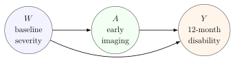
A simplified causal story for early imaging. Baseline factors may affect both imaging and later disability.

The diagram is not a conclusion from the data. It is a scientific description of what might be happening. The arrow \(W\to A\) says that baseline factors influence the probability of imaging. The arrow \(W\to Y\) says that the same or related baseline factors influence disability. The arrow \(A\to Y\) is the possible causal effect of imaging that motivates the study.

8.2 Associative Analysis

An associative analysis summarizes relationships in the observed population. For example, one might compare \[\mathbb{E}(Y\,\vert\,A=1) \quad\text{and}\quad \mathbb{E}(Y\,\vert\,A=0),\] the average disability score among patients who were observed to receive early imaging and the average disability score among patients who were observed not to receive early imaging.

Definition 8.1 (Association). An association is a contrast between features of the observed data distribution, such as \[\mathbb{E}(Y\,\vert\,A=1)-\mathbb{E}(Y\,\vert\,A=0).\] It describes how outcomes differ between groups as they actually occurred.

The observed mean difference \[\mathbb{E}(Y\,\vert\,A=1)-\mathbb{E}(Y\,\vert\,A=0)\] is meaningful as a descriptive parameter. It answers: among patients in the target population, how do observed outcomes differ between those who did and did not receive early imaging?

It does not by itself answer: what would happen if the imaging decision were changed? If patients receiving early imaging tend to have worse baseline symptoms, then the observed imaging group may have worse later disability even if imaging itself has no harmful effect.

8.3 Causal Analysis

Causal analysis asks questions about populations under interventions. Instead of comparing patients as they happened to be treated, we compare hypothetical worlds in which treatment assignment is deliberately changed.

Definition 8.2 (Causal analysis). A causal analysis targets a feature of a population under one or more interventions. For a binary treatment \(A\), a causal analysis might compare the mean outcome if everyone received \(A=1\) with the mean outcome if everyone received \(A=0\).

For the back pain example, the causal question might be:

What would be the average 12-month disability score if all eligible older adults with a new primary care visit for back pain received early imaging, compared with if none received early imaging?

This question is not merely about the subgroup who actually received imaging. It is about the same target population under two alternative interventions.

Key Idea

Associative analysis compares observed groups. Causal analysis compares intervention-generated worlds.

8.4 Population under Intervention

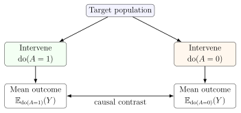
To formalize the difference, imagine two intervention regimes: \[\operatorname{do}(A=1): \text{ assign everyone to early imaging},\] and \[\operatorname{do}(A=0): \text{ assign everyone to no early imaging}.\] The notation \(\operatorname{do}(A=a)\) emphasizes that the treatment value is set by intervention rather than merely observed.

Let \(\mathbb{E}_{\operatorname{do}(A=1)}(Y)\) denote the mean disability score in the population under the intervention assigning everyone to early imaging. Let \(\mathbb{E}_{\operatorname{do}(A=0)}(Y)\) denote the corresponding mean under no early imaging. A causal contrast is \[\mathbb{E}_{\operatorname{do}(A=1)}(Y)-\mathbb{E}_{\operatorname{do}(A=0)}(Y).\]

A causal contrast compares the same population under different interventions.

8.5 Why Data Alone Cannot Answer Causal Questions

The observed data contain outcomes under the treatment decisions that actually occurred. They do not automatically contain outcomes under alternative treatment policies. If a patient received imaging, we observe that patient’s outcome after imaging. We do not also observe that same patient’s outcome under no imaging at the same time and in the same circumstances.

This is the central reason causal inference requires assumptions. The data may show that early imaging patients had higher health care utilization. That observed association could reflect a causal effect of imaging, but it could also reflect that patients selected for imaging had more severe or concerning presentations.

Randomized trials help because the treatment assignment mechanism is controlled by design. Even then, the causal question may go beyond the literal trial data. Participants may not adhere to assigned treatment, clinicians may deviate from protocol, and follow-up may be incomplete. A question such as "what would happen if everyone complied and no one dropped out?" still refers to a hypothetical intervention.

8.6 Untestable Assumptions

Causal Assumption

Causal inference from observational data, and from many randomized trials with nonadherence or missingness, requires assumptions that cannot be verified from the observed data distribution alone. These assumptions connect observed outcomes to outcomes that would have been seen under interventions.

Untestable does not mean arbitrary. Good causal assumptions come from design knowledge, biology, clinical expertise, institutional knowledge, measurement details, and transparent reasoning. The point is that the observed data distribution cannot, by itself, distinguish all causal explanations that generate the same associations.

For the early imaging example, investigators must reason about questions such as:

Which baseline factors influence a clinician’s decision to order imaging?
Which baseline factors also influence later disability or health care use?
Were those factors measured well enough to compare like with like?
Is "early imaging" a sufficiently precise intervention?

The rest of the course develops a formal language for asking these questions, stating the necessary assumptions, and determining when causal parameters can be learned from observed data.

Lecture 2.2. The Roadmap for Causal Analysis

9.1 Overview

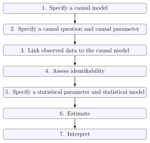
Causal analysis is easiest to learn as a sequence of distinct tasks. Mixing these tasks is a common source of confusion. For example, fitting a regression model before defining the causal question often leads to interpreting a convenient coefficient rather than estimating a meaningful causal parameter.

Key Idea

The causal roadmap separates scientific definition, causal identification, statistical estimation, and interpretation. Each step answers a different question.

A practical roadmap for causal analysis.

9.2 Specify a Causal Model

A causal model represents scientific knowledge about how variables in the system relate to one another. At this stage we ask questions such as:

What factors affect whether a patient receives early imaging?
What factors affect later disability?
Which variables occur before treatment, during follow-up, or after the outcome?
Which important causes were not measured?

In this course, causal models will often be represented by directed acyclic graphs (DAGs) and single world intervention graphs (SWIGs). The graph is not just a picture. It encodes assumptions about causes, noncauses, and conditional independencies.

9.3 Specify a Causal Question and Parameter

The causal question must state the intervention and the outcome. A vague question such as "Does imaging help?" is not yet a causal parameter. A more precise version is:

Among older adults with a new primary care visit for back pain, what is the difference in mean 12-month disability if everyone received lumbar imaging within six weeks versus if no one received lumbar imaging within six weeks?

Using potential outcome notation, this question could be represented by \[\psi=\mathbb{E}\{Y(1)\}-\mathbb{E}\{Y(0)\},\] where \(Y(1)\) is the outcome that would be observed under early imaging and \(Y(0)\) is the outcome that would be observed under no early imaging.

Definition 9.1 (Causal parameter). A causal parameter is a summary of the distribution of counterfactual variables in a target population. It is the causal estimand.

9.4 Link Observed Data to the Causal Model

The causal model describes variables that may include both observed and unobserved quantities. The observed data describe what was actually measured. A common observed data structure for a point-treatment study is \[O=(W,A,Y),\] where \(W\) denotes baseline covariates, \(A\) observed treatment, and \(Y\) observed outcome.

The analyst must state how these observed variables correspond to nodes in the causal model. If the graph contains an unmeasured severity variable \(U\), the observed data do not include \(U\). If the graph contains a broad baseline node \(W\), the analyst must clarify which measured variables are included in \(W\).

This step also includes assumptions that connect observed outcomes to counterfactual outcomes, especially consistency, introduced later in this chapter.

9.5 Assess Identifiability

Identification asks whether the causal parameter can be expressed as a function of the observed data distribution under the stated causal model.

Definition 9.2 (Identifiability). A causal parameter is identifiable from the observed data distribution under a set of assumptions if all causal models satisfying those assumptions and producing the same observed data distribution imply the same value of the causal parameter.

Plainly, identifiability asks: if we had infinite observed data from this study design, would the causal question be answerable? This question comes before estimation. No estimator, no matter how flexible, can recover a causal parameter that is not identified without additional assumptions.

Identification Result

Identification is the bridge from counterfactual quantities to observed-data quantities. A typical goal is to replace a causal expression such as \(\mathbb{E}\{Y(a)\}\) with an observed-data expression such as \(\mathbb{E}\{\mathbb{E}(Y\,\vert\,A=a,W)\}\) under appropriate assumptions.

9.6 Specify Statistical Parameter and Model

Once a causal parameter has been identified, the target becomes a statistical parameter of the observed data distribution. For example, an identification result might show that \[\mathbb{E}\{Y(a)\}=\mathbb{E}\{\mathbb{E}(Y\,\vert\,A=a,W)\}.\] The right-hand side is an observed-data parameter. It depends on the distribution of \((W,A,Y)\), not directly on unobserved counterfactuals.

The statistical model describes what is assumed about the observed data distribution. A nonparametric model makes few restrictions. A parametric model might assume a specific logistic regression or linear regression form. The choice of statistical model affects estimation and inference, but it is conceptually separate from the causal identification assumptions.

9.7 Estimate

Estimation uses the finite sample to approximate the statistical parameter. If the identified parameter involves the conditional mean \(\mathbb{E}(Y\,\vert\,A=a,W)\), then an estimator may require fitting an outcome regression. If it involves \(\mathbb{P}(A=a\,\vert\,W)\), then an estimator may require fitting a propensity score.

Estimation Notes

The estimation step answers a statistical question: given the identified observed-data parameter and a sample \(O_1,\ldots,O_n\), how should we compute a numerical estimate and quantify uncertainty?

Estimation should not change the estimand. A regression coefficient may be easy to estimate, but it is not automatically the causal parameter. The target parameter should be defined before the estimator is chosen.

9.8 Interpret

The final step translates the estimate back into the scientific question while respecting the assumptions and limitations. Interpretation should state:

the target population;
the intervention being compared;
the outcome and time scale;
the causal assumptions required;
the statistical uncertainty;
limitations from measurement, missing data, adherence, and generalizability.

A careful interpretation might say that the result estimates the mean difference in 12-month disability under two specified imaging policies, among patients represented by the study population, assuming the measured covariates were sufficient to control confounding, treatment was well-defined, and follow-up bias was adequately handled.

Lecture 2.3. Causal Models and DAGs

10.1 Why Graphical Models

Causal questions require assumptions about how variables relate to one another. Graphical models provide a compact way to state those assumptions before analyzing the data.

Graphs are useful for three reasons. First, they force the analyst to name the variables believed to be relevant. Second, they make assumed causal relationships visible. Third, they translate scientific claims into mathematical restrictions that can be studied systematically.

Key Idea

A causal graph is a disciplined way to draw assumptions before drawing conclusions.

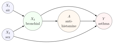
For example, in a study of antihistamine use and asthma incidence among children, suppose:

\(X_1\) is air pollution level;
\(X_2\) is biological sex;
\(X_3\) is bronchial reactivity;
\(A\) is antihistamine treatment;
\(Y\) is asthma incidence.

Subject-matter knowledge may suggest that pollution influences bronchial reactivity and antihistamine use, sex influences bronchial reactivity and asthma, and antihistamine use may influence asthma.

10.2 Directed Acyclic Graphs

Definition 10.1 (Directed acyclic graph). A directed acyclic graph (DAG) is a graph consisting of nodes and directed edges, with no directed cycle. A directed cycle is a path following arrow directions that starts and ends at the same node.

"Directed" means arrows have arrowheads. "Acyclic" means a variable cannot be its own cause through a sequence of arrows such as \(A\to B\to C\to A\).

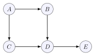
A directed acyclic graph with five nodes.

10.3 Nodes and Edges

Definition 10.2 (Nodes and edges). The nodes or vertices of a DAG represent variables. A directed edge \(X\to Y\) is an arrow from node \(X\) to node \(Y\). Two nodes are adjacent if they are connected by an edge.

A node can represent a scalar variable, such as treatment \(A\), or a vector of variables, such as \[W=(W_1,\ldots,W_{30}),\] where \(W\) is a baseline survey with 30 items. Whether variables should be collapsed into one node depends on the scientific question. If one survey item is the exposure of interest, it should not be hidden inside a broad \(W\) node.

10.4 Parents, Children, Ancestors, Descendants

Definition 10.3 (Family relationships in a DAG). If \(X\to Y\), then \(X\) is a parent of \(Y\) and \(Y\) is a child of \(X\). An ancestor of \(Y\) is any node with a directed path into \(Y\). A descendant of \(X\) is any node reached by a directed path out of \(X\).

In the five-node graph above, \[\mathop{\mathrm{pa}}(D)=\{B,C\}, \qquad \mathop{\mathrm{ch}}(A)=\{B,C\}.\] The ancestors of \(E\) are \(A,B,C,D\), and the descendants of \(A\) are \(B,C,D,E\).

10.5 Causal Meaning of Arrows

A causal DAG gives arrows a causal interpretation. An arrow \(X\to Y\) means that \(X\) is a direct cause of \(Y\) relative to the variables included in the graph.

"Direct" is relative to the graph. If \(X\to M\to Y\) and there is no arrow \(X\to Y\), the graph says that \(X\) may affect \(Y\) through \(M\) but has no direct effect on \(Y\) not mediated by \(M\), among the variables represented.

For the antihistamine example, one possible DAG is:

A possible causal DAG for antihistamine treatment and asthma.

10.6 Meaning of Absent Arrows

Absent arrows are as important as present arrows. If a causal DAG omits \(X\to Y\), it asserts that \(X\) has no direct causal effect on \(Y\) once the other variables in the graph are included.

For example, if the graph includes \(X_1\to X_3\to Y\) but no \(X_1\to Y\), it says that air pollution affects asthma only through the represented intermediate variables, not directly. This is a strong scientific claim.

If the analyst is unsure whether a direct effect exists, a conservative strategy is to leave the arrow in. Removing an arrow encodes knowledge; it should not be done merely to simplify the graph.

10.7 DAGs as Scientific Assumptions

A DAG is not estimated mechanically from the data in the ordinary causal workflow. It represents assumptions supplied by design knowledge and subject-matter reasoning. Data can sometimes contradict implications of a DAG, but many causal features of a DAG are not testable from observed data alone.

Causal Assumption

Using a causal DAG means accepting the causal claims encoded by its arrows and missing arrows. The graph is part of the causal model, not a decorative summary of associations.

DAG construction should therefore be collaborative. Domain experts often know mechanisms that are invisible in a spreadsheet. A useful graph may also reveal discomfort: important variables were not measured, intervention timing is unclear, or some arrows cannot be confidently removed. That discomfort is scientifically productive because it clarifies what the data can and cannot support.

Lecture 2.4. DAGs and Conditional Independencies

11.1 DAG Factorization

DAGs are useful because they connect causal structure to probabilistic structure. For any ordered variables \(A,B,C,D,E\), the chain rule always gives \[\mathbb{P}(A,B,C,D,E) = \mathbb{P}(A)\mathbb{P}(B\,\vert\,A)\mathbb{P}(C\,\vert\,A,B)\mathbb{P}(D\,\vert\,A,B,C)\mathbb{P}(E\,\vert\,A,B,C,D).\] This identity is true for any joint distribution and does not require a graph.

Now consider the DAG \[A\to B,\quad A\to C,\quad B\to D,\quad C\to D,\quad D\to E.\] The parent sets are \[\mathop{\mathrm{pa}}(A)=\emptyset,\quad \mathop{\mathrm{pa}}(B)=\{A\},\quad \mathop{\mathrm{pa}}(C)=\{A\},\quad \mathop{\mathrm{pa}}(D)=\{B,C\},\quad \mathop{\mathrm{pa}}(E)=\{D\}.\] The DAG factorization is \[\mathbb{P}(A,B,C,D,E) = \mathbb{P}(A)\mathbb{P}(B\,\vert\,A)\mathbb{P}(C\,\vert\,A)\mathbb{P}(D\,\vert\,B,C)\mathbb{P}(E\,\vert\,D).\]

Definition 11.1 (DAG factorization). A distribution is said to factorize according to a DAG if its joint density or mass function can be written as \[p(v)=\prod_{j=1}^m p(v_j\,\vert\,\mathop{\mathrm{pa}}(v_j)),\] where \(\mathop{\mathrm{pa}}(v_j)\) denotes the parents of node \(V_j\) in the graph.

When we use a DAG to read conditional independencies, we are assuming that the relevant distribution is Markov with respect to the DAG, equivalently that it satisfies this factorization.

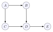
This DAG implies that each node’s distribution depends on its parents, not on all earlier variables.

11.2 Conditional Independence Implied by Missing Arrows

The factorization above removes variables from conditioning sets. For example, the chain rule term \[\mathbb{P}(C\,\vert\,A,B)\] is replaced by \[\mathbb{P}(C\,\vert\,A).\] This replacement encodes \[C\perp\!\!\!\perp B\,\vert\,A.\] Similarly, \[\mathbb{P}(E\,\vert\,A,B,C,D)=\mathbb{P}(E\,\vert\,D)\] encodes that \(E\) is conditionally independent of \(A,B,C\) given \(D\): \[E\perp\!\!\!\perp(A,B,C)\,\vert\,D.\]

Under this Markov/factorization assumption, these conditional independencies follow from missing arrows and the parent structure of the graph. Chapter 3 will introduce d-separation, the graphical rule for reading such independencies systematically.

Key Idea

A DAG does two things at once: it describes causal relationships and implies conditional independence restrictions on the joint distribution.

11.3 Including Measured and Unmeasured Variables

A causal graph should not be restricted to variables that happen to appear in the data set. If an unmeasured factor affects both treatment and outcome, omitting it from the graph hides a threat to causal interpretation.

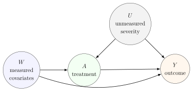
Unmeasured variables should appear in causal graphs when they are part of the scientific system.

The node \(U\) may never be observed, but it matters. If severe symptoms drive both imaging and later disability, then a graph without \(U\) may falsely suggest that measured covariates are sufficient for causal adjustment.

11.4 Collapsing Variables into Nodes

Sometimes a node represents a vector. For instance, \(W\) may stand for age, sex, baseline pain score, comorbidities, insurance status, and prior utilization: \[W=(W_1,\ldots,W_p).\] This is convenient when the internal relationships among the \(W_j\) variables are not central to the causal question.

Collapsing is inappropriate when the relationships inside the vector matter. If one component of \(W\) is the exposure, mediator, or outcome, it should receive its own node. If temporal ordering among components matters, collapsing them can hide causal feedback.

11.5 Representing Time to Avoid Cycles

Many real systems appear cyclic when described coarsely. Infection can cause malnutrition, and malnutrition can increase susceptibility to infection. A DAG cannot contain a cycle, so the solution is to represent the process over time: \[\text{infection}_1 \to \text{malnutrition}_2 \to \text{infection}_3,\] and \[\text{malnutrition}_1 \to \text{infection}_2 \to \text{malnutrition}_3.\]

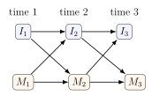
Feedback over time can be represented without cycles by indexing variables by time.

11.6 Building DAGs with Subject-Matter Knowledge

DAG building should start from the scientific system, not from the available columns in the data set. A useful workflow is:

List the exposure, outcome, and variables known or suspected to affect either.
Order variables temporally when possible.
Begin with a rich graph containing plausible arrows.
Remove an arrow only when there is a substantive reason to believe the direct effect is absent.
Mark which variables are measured and which are unmeasured.
Revisit the graph with subject-matter experts.

If the graph shows that key variables were not measured, that is not a failure of graphing. It is useful information. The conclusion may be that the current study needs stronger assumptions, a different target question, sensitivity analysis, or more cautious interpretation as an association.

Lecture 2.5. Counterfactual Variables

12.1 Ideal Experiments

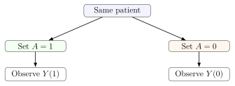
A causal question is easiest to understand by first imagining an ideal experiment. Suppose we want to know whether early imaging affects 12-month back pain-related disability. In an ideal experiment with unlimited control, we could take the target population and create two worlds:

in one world, every eligible patient receives early imaging;
in another world, no eligible patient receives early imaging.

We would then compare the outcomes in these two worlds.

This thought experiment is not meant to be physically possible. Its purpose is to clarify the intervention and the outcome. A causal question is a question about what would happen under actions, not merely about what happened under observed decisions.

Counterfactual thinking compares outcomes for the same unit under alternative interventions.

12.2 Interventions

Definition 12.1 (Intervention). An intervention is an action or policy that sets, modifies, or otherwise changes a variable in the causal system. In notation, \(\operatorname{do}(A=a)\) denotes an intervention setting \(A\) to value \(a\).

An intervention is not the same as conditioning. The expression \(\mathbb{E}(Y\,\vert\,A=a)\) describes the mean outcome among people who were observed with \(A=a\). The expression \(\mathbb{E}\{Y(a)\}\) describes the mean outcome that would be observed if the intervention set \(A=a\) for the relevant population.

Conditioning selects a subgroup. Intervening changes the data-generating process.

12.3 Potential Outcomes \(Y(a)\)

Definition 12.2 (Potential outcome). For a treatment or exposure \(A\) and outcome \(Y\), the potential outcome \(Y(a)\) is the outcome that would be observed for a unit under an intervention setting \(A=a\).

The notation \(Y(a)\) is also called counterfactual notation. It is "counterfactual" when \(a\) differs from the treatment value actually received, but it is useful to define potential outcomes for all intervention levels regardless of what was observed.

If \(A\) is early imaging and \(Y\) is 12-month disability, then: \[Y(1)= \text{disability that would be observed if the patient received early imaging},\] \[Y(0)= \text{disability that would be observed if the patient did not receive early imaging}.\]

12.4 Binary Treatment Potential Outcomes

For a binary treatment \(A\in\{0,1\}\), each unit has two potential outcomes: \[Y(0),\qquad Y(1).\] The observed data contain only one observed outcome \(Y\). If the patient actually received \(A=1\), then under consistency we observe \(Y(1)\). If the patient actually received \(A=0\), then we observe \(Y(0)\). The other potential outcome remains unobserved.

\[\begin{array}{c|ccc} \text{patient} & A & Y(1)& Y(0)\\ \hline 1 & 1 & 1 & 1\\ 2 & 0 & 0 & 0\\ 3 & 0 & 0 & 1\\ 4 & 1 & 1 & 0\\ 5 & 1 & 1 & 0 \end{array}\]

The table is conceptual. In real observed data, both potential outcome columns are not jointly observed for every patient.

12.5 No Interference

The notation \(Y(a)\) assumes that one unit’s potential outcome depends only on that unit’s assigned treatment level, not on treatments assigned to other units.

Causal Assumption

No interference. For unit \(i\), the potential outcome under treatment \(a\) is \(Y_i(a)\) and does not depend on the treatment values assigned to other units: \[Y_i(a_1,\ldots,a_n)=Y_i(a_i)\] for all treatment vectors \((a_1,\ldots,a_n)\), whenever the simplified notation is used.

Plainly, no interference says that my outcome under treatment does not change depending on your treatment.

12.6 Interference Examples

No interference can fail in infectious disease studies. Suppose households contain two people and \(A_i\) indicates flu vaccination for person \(i\). Person 1’s flu infection outcome may depend on whether person 2 is vaccinated. Then the relevant potential outcome is \[Y_1(a_1,a_2),\] not merely \(Y_1(a_1)\).

For a two-person household, the potential outcomes for person 1 might include \[Y_1(1,1),\quad Y_1(1,0),\quad Y_1(0,1),\quad Y_1(0,0).\] The second argument matters because vaccinating the housemate could reduce exposure to infection.

Interference can also arise through social networks, classrooms, neighborhoods, clinics, or markets. Vaccines, infectious disease transmission, peer education, and price interventions are common examples.

12.7 Individual Causal Effects

Definition 12.3 (Individual causal effect). For a binary treatment, an individual causal effect is a contrast between the two potential outcomes for the same unit, such as \[Y_i(1)-Y_i(0)\] or, when meaningful, \[\frac{Y_i(1)}{Y_i(0)}.\]

For a binary adverse outcome, four qualitative types are possible: \[\begin{array}{c|ccc} \text{type} & Y_i(1) & Y_i(0) & Y_i(1)-Y_i(0)\\ \hline \text{doomed} & 1 & 1 & 0\\ \text{invincible} & 0 & 0 & 0\\ \text{helped} & 0 & 1 & -1\\ \text{harmed} & 1 & 0 & 1 \end{array}\] This table is conceptually useful, but it also reveals the central difficulty.

12.8 Fundamental Problem of Causal Inference

Definition 12.4 (Fundamental problem of causal inference). For a given unit at a given time, we can observe the outcome under the treatment actually received, but not under all alternative treatment levels. Therefore individual causal effects are generally not directly observable.

If a patient receives early imaging, we observe the patient’s outcome under imaging. We do not observe the same patient’s outcome at the same time under no imaging. This is why causal inference usually targets population-level summaries rather than individual causal effects.

Key Idea

The causal problem is missing data at the level of potential outcomes. Each unit has multiple potential outcomes, but the observed data reveal at most one of them.

Lecture 2.6. Causal Parameters and Causal Effects

13.1 Population-Level Causal Parameters

Because individual causal effects are generally unobservable, causal inference usually focuses on population-level summaries of potential outcomes.

Definition 13.1 (Population-level causal parameter). A population-level causal parameter is a summary of the distribution of one or more potential outcomes in a target population.

Examples include: \[\mathbb{E}\{Y(1)\},\qquad \mathbb{E}\{Y(0)\},\qquad \mathbb{P}(Y(1)=1),\qquad \operatorname{median}\{Y(1)\}.\] These are not summaries of the observed treatment groups. They are summaries of outcomes under specified interventions.

13.2 Average Causal Effect

The most common causal effect compares average potential outcomes under two interventions.

Definition 13.2 (Average causal effect). For two treatment levels \(a\) and \(a'\), the average causal effect on the additive scale is \[\mathbb{E}\{Y(a)\}-\mathbb{E}\{Y(a')\}.\]

For the early imaging example, the average causal effect of imaging versus no imaging on disability is \[\mathbb{E}\{Y(1)\}-\mathbb{E}\{Y(0)\}.\] If higher values of \(Y\) indicate worse disability, then a positive value means the mean disability would be higher under early imaging than under no early imaging. A negative value means the mean disability would be lower under early imaging.

13.3 Average Treatment Effect

For binary treatment, the average causal effect is often called the average treatment effect.

Definition 13.3 (Average treatment effect). For binary treatment \(A\in\{0,1\}\), the average treatment effect is \[\operatorname{ATE}=\mathbb{E}(Y(1)-Y(0)).\] When expectations are finite, \[\operatorname{ATE}=\mathbb{E}(Y(1))-\mathbb{E}(Y(0)).\]

The second equality is a consequence of linearity of expectation: \[\mathbb{E}(Y(1)-Y(0)) =\mathbb{E}(Y(1))+\mathbb{E}(-Y(0)) =\mathbb{E}(Y(1))-\mathbb{E}(Y(0)).\] This equality is important because it shows that the ATE can be expressed using the two marginal mean potential outcomes.

13.4 Marginal Distributions of Counterfactuals

The ATE depends only on the marginal distributions of \(Y(1)\) and \(Y(0)\). To see this, suppose the potential outcomes are discrete. Then \[\mathbb{E}(Y(1)-Y(0)) = \sum_{y_0}\sum_{y_1}(y_1-y_0) \mathbb{P}(Y(1)=y_1,Y(0)=y_0).\] Distribute the sum: \[= \sum_{y_0}\sum_{y_1}y_1\mathbb{P}(Y(1)=y_1,Y(0)=y_0) - \sum_{y_0}\sum_{y_1}y_0\mathbb{P}(Y(1)=y_1,Y(0)=y_0).\] For the first term, move \(y_1\) outside the sum over \(y_0\): \[\sum_{y_1}y_1\sum_{y_0}\mathbb{P}(Y(1)=y_1,Y(0)=y_0) = \sum_{y_1}y_1\mathbb{P}(Y(1)=y_1) = \mathbb{E}(Y(1)).\] For the second term, \[\sum_{y_0}y_0\sum_{y_1}\mathbb{P}(Y(1)=y_1,Y(0)=y_0) = \sum_{y_0}y_0\mathbb{P}(Y(0)=y_0) = \mathbb{E}(Y(0)).\] Therefore \[\mathbb{E}(Y(1)-Y(0))=\mathbb{E}(Y(1))-\mathbb{E}(Y(0)).\]

Identification Result

This derivation is not yet an identification result from observed data. It is a counterfactual distribution result: the additive ATE depends only on the marginal distributions of \(Y(1)\) and \(Y(0)\), not on their joint distribution.

13.5 Cross-World Quantities

Some causal quantities depend on the joint distribution of potential outcomes under incompatible interventions. For example, \[\mathbb{E}\left(\frac{Y(1)}{Y(0)}\right)\] requires the pair \((Y(1),Y(0))\) for the same unit.

For discrete potential outcomes, \[\mathbb{E}\left(\frac{Y(1)}{Y(0)}\right) = \sum_{y_0}\sum_{y_1} \frac{y_1}{y_0} \mathbb{P}(Y(1)=y_1,Y(0)=y_0),\] when the ratio is well-defined. This expression depends on the joint probabilities \(\mathbb{P}(Y(1)=y_1,Y(0)=y_0)\), not merely the separate marginal distributions.

13.6 Why Cross-World Assumptions Are Problematic

The problem is that no ordinary experiment can observe both \(Y(1)\) and \(Y(0)\) for the same unit at the same time. An experiment assigning everyone to \(A=1\) can reveal features of the distribution of \(Y(1)\). An experiment assigning everyone to \(A=0\) can reveal features of the distribution of \(Y(0)\). Neither experiment reveals how \(Y(1)\) and \(Y(0)\) are paired within individuals.

Any claim about their joint distribution requires assumptions linking outcomes across mutually exclusive worlds. These are called cross-world assumptions. Such assumptions may be mathematically convenient, but they are often difficult to justify scientifically.

Key Idea

Causal parameters based on marginal distributions of potential outcomes are usually preferable because they correspond more directly to ideal experiments. Parameters requiring the joint distribution of incompatible potential outcomes demand stronger cross-world assumptions.

13.7 Risk Differences, Ratios, and Other Contrasts

When \(Y\) is binary, \(\mathbb{E}\{Y(a)\}=\mathbb{P}\{Y(a)=1\}\) is the risk under intervention \(a\). Several contrasts are common: \[\text{Risk difference}= \mathbb{P}(Y(1)=1)-\mathbb{P}(Y(0)=1),\] \[\text{Risk ratio}= \frac{\mathbb{P}(Y(1)=1)}{\mathbb{P}(Y(0)=1)},\] \[\text{Odds ratio}= \frac{\mathbb{P}(Y(1)=1)/\mathbb{P}(Y(1)=0)} {\mathbb{P}(Y(0)=1)/\mathbb{P}(Y(0)=0)}.\]

For continuous outcomes, one may compare means, medians, variances, quantiles, or probabilities of exceeding a clinically meaningful threshold: \[\mathbb{P}(Y(1)>c)-\mathbb{P}(Y(0)>c).\] The best contrast depends on the scientific question, the outcome scale, and interpretability.

Lecture 2.7. Marginal and Conditional Causal Effects

14.1 Marginal ATE

The marginal average treatment effect summarizes the effect in the entire target population: \[\operatorname{ATE}=\mathbb{E}(Y(1)-Y(0)).\] It averages over all sources of variation in the population, including baseline covariates. In the early imaging example, the marginal ATE answers:

What is the average difference in disability if everyone in the target population received early imaging versus if no one received early imaging?

The marginal ATE is often the primary public health or policy estimand because it describes the average impact of a population-level intervention.

14.2 Conditional ATE

A conditional average treatment effect restricts the comparison to a subgroup defined by covariates.

Definition 14.1 (Conditional average treatment effect). For covariates \(W\), the conditional average treatment effect at covariate value \(w\) is \[\operatorname{CATE}(w)=\mathbb{E}(Y(1)-Y(0)\,\vert\,W=w).\]

If \(W\) is baseline pain severity, then \(\operatorname{CATE}(w)\) is the average effect of early imaging among patients with baseline pain severity \(w\).

14.3 Subgroup-Specific Causal Effects

Subgroup-specific causal effects are conditional effects for scientifically meaningful groups. If \(W\) is categorical, such as low, moderate, and severe baseline pain, then \[\mathbb{E}(Y(1)-Y(0)\,\vert\,W=\text{severe})\] is the ATE among patients with severe baseline pain.

The marginal ATE is a weighted average of conditional ATEs: \[\operatorname{ATE} =\mathbb{E}\{\mathbb{E}(Y(1)-Y(0)\,\vert\,W)\}.\] For discrete \(W\), \[\operatorname{ATE} = \sum_w \mathbb{E}(Y(1)-Y(0)\,\vert\,W=w)\mathbb{P}(W=w).\] This is the tower rule applied to the individual-level contrast \(Y(1)-Y(0)\).

14.4 Causal Effect Modification

Definition 14.2 (Causal effect modification). There is causal effect modification by \(W\) on the additive scale if \[\mathbb{E}(Y(1)-Y(0)\,\vert\,W=w)\] varies with \(w\).

For example, early imaging might have little average effect among patients with mild baseline pain but a different effect among patients with severe neurological symptoms. If the conditional causal effect differs across baseline severity levels, severity modifies the causal effect.

Example 14.3 (A finite population). Suppose a population of ten individuals has potential outcomes shown below. \[\begin{array}{c|ccc|c} \text{ID} & W & Y(1)& Y(0)& Y(1)-Y(0)\\ \hline 1 & 2 & 2 & 3 & -1\\ 2 & 1 & 10 & 5 & 5\\ 3 & 1 & 8 & 7 & 1\\ 4 & 1 & 6 & 3 & 3\\ 5 & 0 & 2 & 0 & 2\\ 6 & 2 & 3 & 6 & -3\\ 7 & 0 & 4 & 0 & 4\\ 8 & 1 & 0 & 5 & -5\\ 9 & 2 & 7 & 0 & 7\\ 10 & 0 & 6 & 9 & -3 \end{array}\] The marginal ATE is the average of the ten individual contrasts: \[\operatorname{ATE}=\frac{-1+5+1+3+2-3+4-5+7-3}{10}=1.\] The conditional effects are \[\operatorname{CATE}(0)=\frac{2+4-3}{3}=1,\] \[\operatorname{CATE}(1)=\frac{5+1+3-5}{4}=1,\] \[\operatorname{CATE}(2)=\frac{-1-3+7}{3}=1.\] In this example the marginal and subgroup effects are all equal on the additive scale, so there is no additive effect modification by \(W\).

14.5 Difference between Statistical Interaction and Causal Effect Heterogeneity

Statistical interaction refers to variation in an observed-data association across levels of a covariate. For example, a regression model might show that \[\mathbb{E}(Y\,\vert\,A=1,W=w)-\mathbb{E}(Y\,\vert\,A=0,W=w)\] varies with \(w\).

Causal effect heterogeneity refers to variation in a counterfactual contrast: \[\mathbb{E}(Y(1)-Y(0)\,\vert\,W=w).\] These are not the same object. Observed statistical interactions can arise from confounding, selection, measurement, or model scale. Conversely, causal effect heterogeneity can exist even when a particular regression model fails to show an interaction.

Key Idea

Effect modification is scale-specific and causal. It concerns whether a causal contrast, such as a risk difference or mean difference, varies across subgroups.

Lecture 2.8. From DAGs to SWIGs

15.1 Single World Intervention Graphs

DAGs represent causal relationships among observed or naturally occurring variables. Potential outcomes such as \(Y(a)\) do not appear directly on an ordinary DAG. Single World Intervention Graphs, or SWIGs, extend DAGs so that counterfactual variables can be represented graphically.

Definition 15.1 (Single World Intervention Graph). A Single World Intervention Graph is a graph obtained from a causal DAG by splitting intervention nodes into a random part and a fixed intervention part, then relabeling downstream variables as counterfactual variables under that intervention.

"Single world" emphasizes that the graph represents one intervention world at a time. A SWIG for \(A=1\) and a SWIG for \(A=0\) are distinct intervention worlds.

15.2 Splitting Treatment Nodes

Suppose the original DAG is \[W\to A\to Y,\qquad W\to Y.\] To construct the SWIG for intervention \(A=a\), split the node \(A\) into:

a random part \(A\), representing the treatment the unit would naturally receive;
a fixed part \(a\), representing the value imposed by intervention.

Incoming arrows into \(A\) go to the random part. Outgoing arrows from \(A\) leave the fixed part.

A DAG is converted to a SWIG by splitting the intervened treatment node.

15.3 Fixed Intervention Nodes

The fixed node \(a\) is not random. It represents the intervention value. Because it is fixed by the analyst’s hypothetical intervention, it has no probability distribution in the intervention world.

The fixed node inherits outgoing arrows from the original treatment node. If \(A\) had an arrow to \(Y\) in the DAG, then \(a\) has an arrow to \(Y(a)\) in the SWIG. If \(A\) had an arrow to a mediator \(M\), then \(a\) has an arrow to the counterfactual mediator \(\mathcal{M}(a)\).

15.4 Random Counterfactual Nodes

Downstream nodes are relabeled as counterfactuals. If \(Y\) is downstream of \(A\), then under intervention \(A=a\) the outcome node becomes \(Y(a)\). If \(M\) is downstream of \(A\), it becomes \(M(a)\).

Nodes not downstream of the intervention keep their original labels. In the graph above, \(W\) is a baseline covariate before \(A\), so it remains \(W\).

15.5 Constructing SWIGs from DAGs

The construction rule is:

Start with a causal DAG.
Choose the node or nodes to intervene on.
Split each intervention node into a random part and fixed part.
Send incoming arrows to the random part.
Send outgoing arrows from the fixed part.
Relabel downstream nodes as counterfactual variables under the intervention.

For a mediation DAG \(A\to M\to Y\) with also \(A\to Y\), intervening on \(A=a\) gives:

A mediation DAG and the SWIG under intervention \(A=a\).

If we intervene on both treatment and mediator, setting \(A=a\) and \(M=m\), the downstream outcome becomes \(Y(a,m)\).

15.6 Reading Counterfactual Quantities from SWIGs

SWIGs help identify which counterfactual variables are generated by a particular intervention. In the simple treatment graph, the SWIG for \(A=a\) contains \(Y(a)\), so \(\mathbb{E}\{Y(a)\}\) is a natural causal parameter.

In the mediation graph, the SWIG for \(A=a\) contains \(M(a)\) and \(Y(a)\). A SWIG for the joint intervention \((A=a,M=m)\) contains \(Y(a,m)\). These are different causal questions: \[Y(a) \quad\text{allows the mediator to respond naturally to } A=a,\] whereas \[Y(a,m) \quad\text{sets both treatment and mediator}.\]

Key Idea

SWIGs make the intervention explicit. Different interventions on the same original DAG can generate different counterfactual variables and therefore different causal questions.

Lecture 2.9. Types of Interventions and Consistency

16.1 Static Interventions

The simplest interventions are static interventions.

Definition 16.1 (Static intervention). A static intervention assigns the same fixed treatment value or treatment regime to every unit in the target population.

For a binary point treatment, examples are: \[\operatorname{do}(A=1): \text{ assign everyone to treatment},\] \[\operatorname{do}(A=0): \text{ assign everyone to no treatment}.\] The corresponding potential outcomes are \(Y(1)\) and \(Y(0)\).

Not all interventions are static. A stochastic intervention assigns treatment according to a specified probability distribution. A dynamic intervention assigns treatment according to a rule depending on a person’s evolving history. For example, an HIV treatment rule might switch therapy when CD4 count falls below a threshold.

16.2 Well-Defined Interventions

A causal question is only as clear as its intervention.

Definition 16.2 (Well-defined intervention). An intervention is well-defined if it specifies the action sufficiently clearly that the relevant potential outcome has a stable meaning across units and settings.

"Early imaging" may be ambiguous. Does it mean recommending imaging, ordering imaging, completing imaging, obtaining MRI only, obtaining any lumbar imaging, or ensuring imaging within a particular number of days? These versions may have different effects.

Similarly, "the effect of BMI" is ambiguous unless the intervention is specified. Reducing BMI by diet, exercise, medication, or surgery may have different biological and social consequences. A causal question should describe the action, not only the variable label.

Causal Assumption

When using potential outcome notation \(Y(a)\), we assume that the intervention level \(a\) is defined clearly enough that the counterfactual outcome is meaningful. Ambiguous treatment versions can make consistency and interpretation fail.

16.3 Hypothetical Interventions

Some interventions are hypothetical but still useful. A policy may not yet exist, or a trial may not be feasible, but the intervention can be described coherently enough to define a causal parameter.

For example, one might ask what would happen if all eligible patients received a reminder phone call, even if such a reminder system has not yet been implemented. The intervention is hypothetical but imaginable.

Other questions are more difficult. Asking for "the causal effect of race" is problematic if no well-defined intervention on race is specified. More precise questions may target interventions on discriminatory treatment, names on resumes, neighborhood assignment, income, educational access, or other manipulable social conditions. These questions may not capture every meaning of race, but they define clearer intervention contrasts.

16.4 Manipulability

Some scholars argue that causal effects should be defined only for variables that are manipulable. Others allow causal questions about nonmanipulable attributes if the counterfactual contrast is scientifically meaningful and carefully interpreted.

The practical lesson is not that every variable must be physically manipulable in a laboratory. The lesson is that the analyst must say what intervention, policy, or hypothetical change gives meaning to the potential outcome.

Key Idea

Causal inference is about effects of interventions. When the intervention is vague, the causal parameter is vague.

16.5 Causal Consistency

Consistency links potential outcomes to observed outcomes.

Causal Assumption

Causal consistency. If a unit is observed to receive treatment level \(A=a\), then its observed outcome equals its potential outcome under that treatment level: \[Y=Y(a)\quad\text{for units with }A=a.\] For binary treatment, this can be written as \[Y=AY(1)+(1-A)Y(0).\]

The binary formula is worth unpacking. If \(A=1\), then \[AY(1)+(1-A)Y(0)=1\cdot Y(1)+0\cdot Y(0)=Y(1).\] If \(A=0\), then \[AY(1)+(1-A)Y(0)=0\cdot Y(1)+1\cdot Y(0)=Y(0).\] Thus the formula says exactly that the observed outcome is the potential outcome corresponding to the treatment actually received.

Example 16.3 (Observed and ideal data). In an ideal data table for binary treatment, each patient has \(A\), \(Y(0)\), and \(Y(1)\): \[\begin{array}{c|ccc} \text{ID} & A & Y(0)& Y(1)\\ \hline 1 & 1 & 1 & 0\\ 2 & 0 & 0 & 0\\ 3 & 0 & 1 & 1\\ 4 & 1 & 0 & 1 \end{array}\] The observed data contain \(A\) and \(Y\): \[\begin{array}{c|cc} \text{ID} & A & Y\\ \hline 1 & 1 & 0\\ 2 & 0 & 0\\ 3 & 0 & 1\\ 4 & 1 & 1 \end{array}\] For each row, the observed \(Y\) equals the potential outcome under the observed treatment.

16.6 Statistical Consistency vs Causal Consistency

Causal consistency is different from statistical consistency. Statistical consistency is a property of an estimator: \[\hat\psi_n \overset{P}{\longrightarrow} \psi.\] It says that, with increasing sample size, the estimator approaches the target parameter.

Causal consistency is an assumption about the relationship between observed outcomes and potential outcomes. It says that the observed outcome under the observed treatment agrees with the corresponding counterfactual outcome.

The two ideas share a word but belong to different parts of the roadmap. Statistical consistency concerns estimation. Causal consistency concerns the definition and linkage of causal and observed data.

16.7 Measured and Unmeasured Variables

Before assessing whether a causal parameter can be identified, the analyst must mark which variables in the causal model are measured. A SWIG or DAG may include:

measured baseline covariates \(W\);
measured treatment \(A\);
measured outcome \(Y\);
unmeasured common causes \(U\);
post-treatment variables \(Z\) or mediators \(M\).

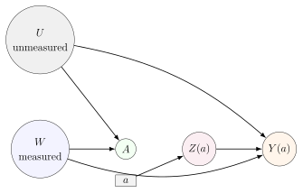
A SWIG can distinguish measured covariates, unmeasured variables, fixed interventions, and counterfactual descendants.

This distinction will matter for identification. If all common causes of treatment and outcome are measured, one set of identification strategies may be plausible. If important common causes are unmeasured, different strategies or stronger assumptions may be required.

Key Idea

Chapter 2 defines the language of causal questions: interventions, potential outcomes, causal parameters, graphs, SWIGs, and consistency. Chapter 3 asks when these causal quantities can be learned from observed data.

Chapter 3. Identification of Causal Parameters and the ATE

Lecture 3.1. What Is Causal Identification?

17.1 Counterfactual Distribution vs Observed Data Distribution

Chapter 2 introduced causal parameters as summaries of counterfactual variables. For a binary treatment \(A\), the average treatment effect is \[\operatorname{ATE}=\mathbb{E}(Y(1)-Y(0))=\mathbb{E}(Y(1))-\mathbb{E}(Y(0)).\] This parameter is defined in terms of the joint scientific object containing potential outcomes. The observed data, however, usually have the form \[O=(W,A,Y),\] where \(W\) denotes measured covariates, \(A\) the treatment actually received, and \(Y\) the outcome actually observed.

Definition 17.1 (Counterfactual distribution). The counterfactual distribution is the probability distribution of variables such as \(Y(0)\), \(Y(1)\), and possibly other counterfactual quantities under interventions.

Definition 17.2 (Observed data distribution). The observed data distribution is the probability distribution of the variables actually measured in the study, such as \(P(W,A,Y)\).

These are different objects. The causal parameter \(\mathbb{E}(Y(1))\) lives in the counterfactual distribution. A statistical parameter such as \(\mathbb{E}\{\mathbb{E}(Y\,\vert\,A=1,W)\}\) lives in the observed data distribution.

17.2 Identification as a Bridge

Identification asks whether a causal parameter can be rewritten using only the observed data distribution, under clearly stated assumptions.

Definition 17.3 (Causal identification). A causal parameter \(\psi\) is identified under a causal model if \(\psi\) is equal to a functional of the observed data distribution \(P(O)\) for every data-generating process satisfying the assumptions in that causal model.

Informally, identification means we can write an equality of the form \[\text{counterfactual quantity} \quad \overset{\text{assumptions}}{=} \quad \text{observed-data quantity}.\] For example, later in this chapter we will derive \[\mathbb{E}\{Y(a)\} = \mathbb{E}\{\mathbb{E}(Y\,\vert\,A=a,W)\},\] under consistency, conditional randomization, and positivity. The left side is causal. The right side is a statistical parameter of the observed distribution.

Identification connects a causal estimand to an observed-data parameter.

17.3 Identifiability in the Causal Roadmap

Identification is the fourth step in the causal roadmap:

specify a causal model;
specify a causal question and causal parameter;
specify observed data and link them to the causal model;
assess identifiability;
specify a statistical parameter and model;
estimate;
interpret.

The ordering matters. Before estimating, we must know what observed-data parameter represents the causal parameter. Otherwise we may estimate a precise but irrelevant quantity.

Identification Result

Identification is a large-sample, infinite-data question. It asks: if we knew the entire observed data distribution exactly, could we determine the causal parameter under the stated assumptions?

17.4 Why Identification Precedes Estimation

Estimation concerns finite-sample uncertainty. Identification concerns whether the target is learnable from the observed data distribution at all. If a causal parameter is not identified, collecting more observations from the same observed data distribution does not solve the problem. Infinite data would reveal the observed distribution perfectly, but the causal parameter could still remain ambiguous.

This distinction is central:

Identification problem: the observed data do not contain enough information, under current assumptions, to determine the causal parameter.
Estimation problem: the causal parameter has been written as an observed-data parameter, and we need to estimate it from a finite sample.

Machine learning can help estimate complex functions such as \(\mathbb{E}(Y\,\vert\,A,W)\) or \(\mathbb{P}(A=1\,\vert\,W)\). It cannot, by itself, create identification. Identification comes from the causal model and assumptions.

Key Idea

Identification tells us what to estimate. Estimation tells us how to approximate that identified statistical target using finite data.

Lecture 3.2. Confounding and Exchangeability

18.1 Classical Confounder Definition

The classical epidemiologic description says that a confounder is a variable associated with both exposure and outcome, and not on the causal pathway from exposure to outcome. For example, baseline disease severity may affect both whether a patient receives a risky cancer treatment and whether the patient dies of cancer. Disease severity can therefore confound the treatment-outcome association.

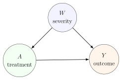
A classical confounding structure: \(W\) is a common cause of treatment and outcome.

This definition is useful but incomplete. In complex problems, variables can be time-varying, affected by prior treatment, measured with error, or unmeasured. A more general definition uses counterfactual independence.

18.2 Counterfactual Independence Definition

Definition 18.1 (No unmeasured confounding for a point treatment). For a binary treatment \(A\), there is no unmeasured confounding given covariates \(W\) if \[Y(0)\perp\!\!\!\perp A \,\vert\,W \qquad\text{and}\qquad Y(1)\perp\!\!\!\perp A \,\vert\,W.\] Equivalently, for \(a\in\{0,1\}\), \[Y(a)\perp\!\!\!\perp A\,\vert\,W.\]

In words, among people with the same covariates \(W\), the treatment actually received carries no additional information about the potential outcomes. Within covariate strata, treated and untreated people are exchangeable with respect to what would happen under either treatment.

18.3 Randomization

In an ideal randomized trial, treatment assignment is generated by a random device that does not use patient prognosis. If treatment is randomized unconditionally, then \[Y(0)\perp\!\!\!\perp A \qquad\text{and}\qquad Y(1)\perp\!\!\!\perp A.\] This means that the treated and untreated groups have the same distribution of potential outcomes before treatment is assigned, up to random sampling variation.

Causal Assumption

Randomization condition. For a binary point treatment, \[Y(a)\perp\!\!\!\perp A,\qquad a=0,1.\] Plainly, treatment assignment gives no information about what the outcome would be under either treatment level.

18.4 Conditional Randomization

In observational studies, unconditional randomization is usually implausible. Treatment decisions often depend on covariates. A weaker assumption is that treatment is randomized within strata of measured covariates: \[Y(a)\perp\!\!\!\perp A\,\vert\,W,\qquad a=0,1.\]

This is plausible when \(W\) contains all common causes of treatment and outcome needed to make treatment assignment as-if random. For example, if physicians choose early imaging based on baseline pain, neurological symptoms, age, cancer history, and prior utilization, then those variables must be included in \(W\) for conditional randomization to be plausible.

Causal Assumption

Conditional randomization. For every treatment level \(a\), \[Y(a)\perp\!\!\!\perp A\,\vert\,W.\] This says treatment is as-if randomized among people with the same \(W\).

18.5 Ignorability

The terms ignorability, conditional ignorability, and no unmeasured confounding are often used for the same counterfactual independence condition. The idea is that after conditioning on \(W\), the treatment assignment mechanism can be ignored for the purpose of identifying the distribution of \(Y(a)\).

The word "ignored" should not be misunderstood. We do not ignore treatment assignment in estimation. Rather, the assumption says that the remaining dependence between treatment and potential outcomes has been removed by conditioning on \(W\).

18.6 Exchangeability

Exchangeability is another name for the same idea, emphasizing comparability of groups.

Definition 18.2 (Exchangeability). Treated and untreated groups are exchangeable with respect to potential outcomes, possibly conditional on \(W\), if their potential outcome distributions are the same: \[Y(a)\perp\!\!\!\perp A\,\vert\,W.\]

If exchangeability holds, then within a stratum \(W=w\), the observed outcomes among people with \(A=a\) can represent the potential outcomes under \(a\) for everyone in that stratum.

18.7 Why Ignorability Cannot Be Empirically Verified

Ignorability involves potential outcomes that are not jointly observed. Among treated people we observe outcomes under treatment, but not what their outcomes would have been without treatment. Among untreated people we observe outcomes without treatment, but not what their outcomes would have been under treatment.

Therefore, the condition \[Y(a)\perp\!\!\!\perp A\,\vert\,W\] cannot be tested directly from the observed data. We can check whether measured covariates are balanced across treatment groups. We can check whether some covariates predict treatment. But we cannot check whether all unmeasured causes of the outcome have been controlled.

Key Idea

Exchangeability is a causal assumption, not an empirical fact discovered by a balance table. Balance diagnostics can reveal problems, but they cannot prove that ignorability holds.

Lecture 3.3. d-Separation in DAGs

19.1 Paths

d-Separation is a graphical rule for reading conditional independence statements from a DAG. It answers questions such as whether \(X\perp\!\!\!\perp Y\,\vert\,Z\) is implied by a graph, under the assumption that the distribution is Markov with respect to the DAG.

Definition 19.1 (Path). A path between two nodes is a sequence of adjacent nodes connecting them, with no node repeated. The arrows on the path do not need to point in the same direction.

For example, in \(A\to B\to D\leftarrow F\), the sequence \(A,B,D,F\) is a path from \(A\) to \(F\), even though the last arrow points into \(D\).

19.2 Forks

A fork has the form \[X\leftarrow Z\to Y.\] Here \(Z\) is a common cause of \(X\) and \(Y\).

A fork: \(X\) and \(Y\) share a common cause \(Z\).

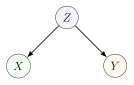
Forks are open unless we condition on the middle node. Thus typically \[X\not\!\perp\!\!\!\perp Y, \qquad X\perp\!\!\!\perp Y\,\vert\,Z\] as implied by this simple graph. Intuitively, warm weather may cause both ice cream sales and visits to the beach. Conditioning on weather removes the common-cause explanation for their association.

19.3 Chains

A chain has the form \[X\to Z\to Y\] or \[X\leftarrow Z\leftarrow Y.\] The middle node transmits association along a directed pathway.

A chain: association flows through the middle node \(Z\).

Chains are open unless we condition on the middle node: \[X\not\!\perp\!\!\!\perp Y, \qquad X\perp\!\!\!\perp Y\,\vert\,Z.\] If \(X\) affects \(Y\) only through \(Z\), then once \(Z\) is known, \(X\) provides no additional information about \(Y\).

19.4 Colliders

A collider has the form \[X\to Z\leftarrow Y.\] The arrows on the path collide at \(Z\).

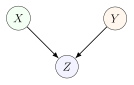
A collider: \(Z\) is a common effect of \(X\) and \(Y\).

Colliders behave differently from forks and chains. A collider blocks the path unless we condition on the collider or one of its descendants: \[X\perp\!\!\!\perp Y, \qquad X\not\!\perp\!\!\!\perp Y\,\vert\,Z.\] For example, a car failing to start may be caused by a dead battery or an empty fuel tank. Before knowing whether the car starts, battery status and fuel status might be independent. After learning the car failed to start, evidence that the battery is fine makes an empty fuel tank more likely.

19.5 Collider Descendants

Conditioning on a descendant of a collider can also open the path. If \[X\to Z\leftarrow Y,\qquad Z\to D,\] then conditioning on \(D\) can induce dependence between \(X\) and \(Y\).

The reason is that \(D\) carries information about the collider \(Z\). If \(D\) is "taken to the mechanic" and \(Z\) is "car fails to start," then observing \(D\) gives partial information about \(Z\), which can create dependence between the causes of \(Z\).

19.6 Blocking and Opening Paths

A path is blocked by a conditioning set \(S\) if at least one of the following occurs:

the path contains a chain or fork whose middle node is in \(S\);
the path contains a collider such that neither the collider nor any descendant of the collider is in \(S\).

Equivalently:

conditioning on non-colliders blocks paths;
conditioning on colliders or their descendants opens paths.

19.7 d-Separation Rules

Definition 19.2 (d-separation). Two nodes \(X\) and \(Y\) are d-separated by a set \(S\) if every path between \(X\) and \(Y\) is blocked by \(S\). If at least one path remains open, \(X\) and \(Y\) are d-connected given \(S\).

If a DAG represents the data-generating process and \(X\) and \(Y\) are d-separated by \(S\), then the graph implies \[X\perp\!\!\!\perp Y\,\vert\,S.\]

19.8 Practice Examples

Consider the DAG: \[A\to B,\quad A\to C,\quad B\to D,\quad C\to D,\quad F\to D,\quad D\to E.\]

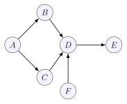
Is \(A\perp\!\!\!\perp E\,\vert\,C\)? No. The path \(A\to B\to D\to E\) remains open.

Is \(A\perp\!\!\!\perp F\)? Yes. The paths \(A\to B\to D\leftarrow F\) and \(A\to C\to D\leftarrow F\) are both blocked at the collider \(D\).

Is \(B\perp\!\!\!\perp C\,\vert\,A\)? Yes. The fork path \(B\leftarrow A\to C\) is blocked by conditioning on \(A\), and the path \(B\to D\leftarrow C\) is blocked by collider \(D\).

Is \(B\perp\!\!\!\perp C\,\vert\,A,D\)? No. Conditioning on collider \(D\) opens \(B\to D\leftarrow C\).

Lecture 3.4. d-Separation in SWIGs

20.1 Paths in SWIGs

SWIGs contain both random nodes and fixed intervention nodes. d-Separation in a SWIG is read using paths among the random nodes, excluding the fixed intervention labels such as \(a\).

Definition 20.1 (Path in a SWIG). A path between two random nodes in a SWIG is a sequence of adjacent random nodes connecting them. Fixed intervention nodes are not included as nodes on the path.

For identification of the ATE, the key graphical question is often whether \[Y(a)\perp\!\!\!\perp A\,\vert\,W\] is implied by the SWIG. This is a statement about independence between the random treatment node \(A\) and the random counterfactual outcome node \(Y(a)\).

20.2 Fixed Intervention Nodes

The fixed node \(a\) represents an intervention setting \(A=a\). It is not random and therefore is not conditioned on in the same way as a random variable. It inherits arrows that leave the original treatment node.

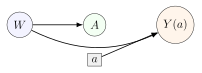
The fixed node \(a\) is not part of random-variable paths, but it defines the intervention world.

The path from \(A\) to \(Y(a)\) through \(W\) is \[A\leftarrow W\to Y(a).\] The arrow from \(a\) to \(Y(a)\) does not create a random path from \(A\) to \(Y(a)\) because \(a\) is fixed.

20.3 Colliders and Non-Colliders in SWIGs

As in DAGs, whether a node is a collider depends on the particular path. A random node \(V\) is a collider on a path if the two adjacent arrows on that path both point into \(V\): \[\cdots \to V \leftarrow \cdots.\] Otherwise, \(V\) is a non-collider on that path.

A node can be a collider on one path and a non-collider on another. Consider paths between \(A\) and \(Y(a)\) in a SWIG with nodes \(W,H,Z\). A node \(Z\) may be a collider on \[Y(a)\leftarrow H\to Z\leftarrow W\to A,\] but a non-collider on \[Y(a)\leftarrow Z\leftarrow A.\] The path determines the role.

20.4 Unconditional d-Separation

A path d-connects two random nodes unconditionally if it has no closed collider and no conditioned non-collider. With no conditioning set, forks and chains are open, while colliders are closed.

Common open unconditional paths include: \[X\to \cdots \to Y, \qquad X\leftarrow \cdots \leftarrow Y, \qquad X\leftarrow \cdots \leftarrow T\to \cdots \to Y.\] The third form is a shared common cause path.

In the SWIG \[A\leftarrow W\to Y(a),\] \(A\) and \(Y(a)\) are not unconditionally d-separated because the fork through \(W\) is open. This represents confounding by \(W\).

20.5 Conditional d-Separation

Definition 20.2 (Conditional d-separation in a SWIG). A path between random nodes is open given a conditioning set \(S\) if every non-collider on the path is not in \(S\), and every collider on the path is either in \(S\) or has a descendant in \(S\). Two nodes are d-separated by \(S\) if every path between them is blocked by \(S\).

This is the same logic as for DAGs, applied to random nodes in the SWIG. Fixed nodes define interventions but are excluded from conditioning sets.

20.6 Reading \(Y(a)\perp\!\!\!\perp A\,\vert\,W\)

The core use of SWIG d-separation in this chapter is to assess conditional randomization. In the confounding SWIG:

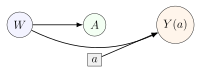
Conditioning on \(W\) blocks the backdoor path from \(A\) to \(Y(a)\).

The only random path between \(A\) and \(Y(a)\) is \[A\leftarrow W\to Y(a).\] This is a fork. Without conditioning, the path is open. Conditioning on \(W\) blocks the path. Therefore the SWIG implies \[Y(a)\perp\!\!\!\perp A\,\vert\,W.\]

Key Idea

In a SWIG, conditional randomization is a d-separation statement between the random treatment node \(A\) and the counterfactual outcome node \(Y(a)\).

If an unmeasured variable \(U\) also points to both \(A\) and \(Y(a)\), then the path \[A\leftarrow U\to Y(a)\] remains open after conditioning on measured \(W\). In that case the graph does not support \(Y(a)\perp\!\!\!\perp A\,\vert\,W\).

Lecture 3.5. Assumptions for Identifying the ATE

21.1 Consistency

To identify the ATE, the observed outcome must be linked to the relevant potential outcome.

Causal Assumption

Consistency. If a unit is observed with \(A=a\), then \[Y=Y(a).\] For binary \(A\), \[Y=AY(1)+(1-A)Y(0).\]

Consistency requires that the treatment versions represented by \(A=a\) are well-defined enough that the observed treatment corresponds to the intervention used to define \(Y(a)\).

21.2 Conditional Randomization

The second assumption is conditional randomization, also called conditional exchangeability or conditional ignorability.

Causal Assumption

Conditional randomization. For \(a\in\{0,1\}\), \[Y(a)\perp\!\!\!\perp A\,\vert\,W.\] Within strata of measured covariates \(W\), the observed treatment carries no information about the potential outcome under treatment level \(a\).

This assumption is usually the hardest to justify in observational studies. It says that \(W\) contains enough information to control confounding.

21.3 Positivity

Even if treatment is as-if randomized within covariate strata, we must have observed treatment variation within those strata.

Causal Assumption

Positivity. For each treatment level \(a\in\{0,1\}\), \[\mathbb{P}(A=a\,\vert\,W=w)>0\] for every covariate value \(w\) with \(\mathbb{P}(W=w)>0\).

In words, every covariate subgroup in the target population must have some chance of receiving each treatment level. If no mildly ill patients ever receive a risky experimental treatment, then the observed data contain no direct information about outcomes under that treatment for mildly ill patients.

21.4 Why Positivity Is Partly Empirically Checkable

Unlike exchangeability, positivity is stated in terms of the observed data distribution. It involves \(\mathbb{P}(A=a\,\vert\,W=w)\), not counterfactual outcomes. Therefore it can be partly checked.

For discrete \(W\), one can inspect whether each covariate stratum contains both treated and untreated observations. For continuous or high-dimensional \(W\), exact strata may be sparse, so analysts examine estimated propensity scores \[g_a(W)=\mathbb{P}(A=a\,\vert\,W)\] and check whether they are close to zero.

Empirical checks are not perfect. A finite sample may fail to show a treatment level in a subgroup even if the population probability is positive. Conversely, a few observations in a subgroup do not guarantee enough information for stable estimation. Still, positivity has observable implications.

21.5 Why Positivity Matters for Observed Conditional Means

The G-computation formula will involve terms such as \[\mathbb{E}(Y\,\vert\,A=a,W=w).\] This conditional mean is defined from the observed data distribution only when \(\mathbb{P}(A=a,W=w)>0\). Since \[\mathbb{P}(A=a,W=w)=\mathbb{P}(A=a\,\vert\,W=w)\mathbb{P}(W=w),\] if \(\mathbb{P}(W=w)>0\) but \(\mathbb{P}(A=a\,\vert\,W=w)=0\), then the subgroup \((A=a,W=w)\) does not exist in the observed population. The conditional mean cannot be learned from observed outcomes.

Key Idea

Exchangeability says treated and untreated people are comparable within \(W\) strata. Positivity says both treated and untreated people actually exist within those strata.

Lecture 3.6. G-Computation Identification Formula

22.1 Derivation of \(\mathbb{E}\{Y(a)\}\)

Assume consistency, conditional randomization, and positivity. For a discrete covariate vector \(W\), begin with the counterfactual mean: \[\mathbb{E}\{Y(a)\}.\] Apply the tower rule by averaging over covariate strata: \[\mathbb{E}\{Y(a)\} = \sum_w \mathbb{E}\{Y(a)\,\vert\,W=w\}\mathbb{P}(W=w).\] Use conditional randomization, \(Y(a)\perp\!\!\!\perp A\,\vert\,W\), to add the event \(A=a\) inside the conditional expectation: \[\mathbb{E}\{Y(a)\,\vert\,W=w\} = \mathbb{E}\{Y(a)\,\vert\,A=a,W=w\}.\] Then use consistency. Among units with \(A=a\), the observed outcome equals \(Y(a)\): \[\mathbb{E}\{Y(a)\,\vert\,A=a,W=w\} = \mathbb{E}(Y\,\vert\,A=a,W=w).\] Substituting gives \[\mathbb{E}\{Y(a)\} = \sum_w \mathbb{E}(Y\,\vert\,A=a,W=w)\mathbb{P}(W=w).\] Equivalently, \[\mathbb{E}\{Y(a)\} = \mathbb{E}\{\mathbb{E}(Y\,\vert\,A=a,W)\}.\]

Identification Result

G-computation identification formula. Under consistency, conditional randomization, and positivity, \[\mathbb{E}\{Y(a)\} = \mathbb{E}\{\mathbb{E}(Y\,\vert\,A=a,W)\}.\] Therefore \[\operatorname{ATE} = \mathbb{E}\{\mathbb{E}(Y\,\vert\,A=1,W)-\mathbb{E}(Y\,\vert\,A=0,W)\}.\]

22.2 Role of the Tower Rule

The tower rule is the first step: \[\mathbb{E}\{Y(a)\} =\sum_w \mathbb{E}\{Y(a)\,\vert\,W=w\}\mathbb{P}(W=w).\] It says that the population mean counterfactual outcome is a weighted average of covariate-specific counterfactual means. The weights are the covariate distribution in the whole target population.

22.3 Role of Conditional Randomization

Conditional randomization justifies replacing the counterfactual mean in the whole \(W=w\) stratum with the counterfactual mean among the observed treatment subgroup: \[\mathbb{E}\{Y(a)\,\vert\,W=w\} = \mathbb{E}\{Y(a)\,\vert\,A=a,W=w\}.\] In words, within the stratum \(W=w\), people who actually received \(A=a\) are representative of everyone in that stratum with respect to \(Y(a)\).

22.4 Role of Consistency

Consistency changes the counterfactual outcome into an observed outcome among those who received \(A=a\): \[\mathbb{E}\{Y(a)\,\vert\,A=a,W=w\} = \mathbb{E}(Y\,\vert\,A=a,W=w).\] This is where the expression becomes fully observed-data based.

22.5 Interpretation as Standardization

The formula \[\sum_w \mathbb{E}(Y\,\vert\,A=a,W=w)\mathbb{P}(W=w)\] standardizes treatment-specific outcome means to the covariate distribution of the whole population.

For each \(w\):

compute the average observed outcome among people with \(A=a\) and \(W=w\);
weight that subgroup mean by the population prevalence \(\mathbb{P}(W=w)\);
sum over all covariate strata.

22.6 G-Computation Intuition

Within each \(W=w\) stratum, conditional randomization makes the observed comparison between \(A=1\) and \(A=0\) fair. The subgroup-specific causal contrast is \[\mathbb{E}(Y\,\vert\,A=1,W=w)-\mathbb{E}(Y\,\vert\,A=0,W=w).\] The population ATE averages these fair subgroup comparisons using the target population distribution of \(W\): \[\operatorname{ATE} = \sum_w \left\{ \mathbb{E}(Y\,\vert\,A=1,W=w)-\mathbb{E}(Y\,\vert\,A=0,W=w) \right\}\mathbb{P}(W=w).\]

22.7 Worked Discrete Example

Let \(Y\) indicate death due to cancer, let \(A=1\) denote a risky treatment and \(A=0\) denote standard treatment, and let \(W=1\) denote severe disease. Consider a population of 320 people with the following observed counts: \[\begin{array}{c|cc|cc} & \multicolumn{2}{c|}{W=0} & \multicolumn{2}{c}{W=1}\\ & A=0 & A=1 & A=0 & A=1\\ \hline Y=1 & 60 & 10 & 30 & 60\\ Y=0 & 60 & 30 & 10 & 60 \end{array}\] Each covariate stratum contains people at both treatment levels, so positivity holds: \[\mathbb{P}(A=a\,\vert\,W=w)>0 \qquad\text{for all }a\in\{0,1\},\;w\in\{0,1\}.\] Suppose conditional randomization and consistency are also valid. Then the observed conditional outcome means identify the stratum-specific counterfactual risks.

For the risky treatment, \[\mathbb{E}(Y\,\vert\,A=1,W=0)=\frac{10}{10+30}=0.25,\] and \[\mathbb{E}(Y\,\vert\,A=1,W=1)=\frac{60}{60+60}=0.50.\] Because the population has 160 people with \(W=0\) and 160 people with \(W=1\), \[\mathbb{P}(W=0)=\mathbb{P}(W=1)=0.50.\] Therefore \[\mathbb{E}\{Y(1)\} =0.25(0.50)+0.50(0.50)=0.375.\] For standard treatment, \[\mathbb{E}(Y\,\vert\,A=0,W=0)=\frac{60}{60+60}=0.50, \qquad \mathbb{E}(Y\,\vert\,A=0,W=1)=\frac{30}{30+10}=0.75,\] so \[\mathbb{E}\{Y(0)\} =0.50(0.50)+0.75(0.50)=0.625.\] The identified ATE on the risk-difference scale is \[\mathbb{E}\{Y(1)\}-\mathbb{E}\{Y(0)\}=0.375-0.625=-0.25.\] Because \(Y=1\) means death, this negative value means the risky treatment lowers the death risk by 25 percentage points in this population under the stated assumptions.

22.8 Why Naive Mean Differences Are Unfair

The naive observed mean difference is \[\mathbb{E}(Y\,\vert\,A=1)-\mathbb{E}(Y\,\vert\,A=0).\] By the tower rule, \[\mathbb{E}(Y\,\vert\,A=1) = \sum_w \mathbb{E}(Y\,\vert\,A=1,W=w)\mathbb{P}(W=w\,\vert\,A=1),\] and \[\mathbb{E}(Y\,\vert\,A=0) = \sum_w \mathbb{E}(Y\,\vert\,A=0,W=w)\mathbb{P}(W=w\,\vert\,A=0).\] Thus the treated mean is averaged over the covariate distribution among treated people, while the untreated mean is averaged over the covariate distribution among untreated people. If treatment groups have different covariate distributions, the comparison mixes treatment differences with covariate-composition differences.

In the cancer example above, the risky treatment group has more severe patients: \[\mathbb{P}(W=1\,\vert\,A=1)=\frac{120}{160}=0.75, \qquad \mathbb{P}(W=1\,\vert\,A=0)=\frac{40}{160}=0.25.\] The naive risks are \[\mathbb{E}(Y\,\vert\,A=1)=\frac{10+60}{160}=0.4375, \qquad \mathbb{E}(Y\,\vert\,A=0)=\frac{60+30}{160}=0.5625,\] so the naive difference is \(-0.125\), only half as large in magnitude as the standardized contrast \(-0.25\). The naive comparison is unfair to the risky treatment because it averages the risky-treatment outcomes over a much sicker covariate distribution.

Key Idea

G-computation keeps the comparison fair by using the same covariate distribution, \(\mathbb{P}(W=w)\), for both treatment levels.

Lecture 3.7. Other Causal Estimands

23.1 Conditional Average Treatment Effect

Suppose \(W=(X,Z)\), where \(X\) defines a subgroup of scientific interest and \(Z\) contains additional covariates needed for confounding control. The conditional average treatment effect as a function of \(X\) is \[\operatorname{CATE}(x)=\mathbb{E}(Y(1)-Y(0)\,\vert\,X=x).\] Under the same consistency, conditional randomization, and positivity assumptions, with randomization conditional on \((X,Z)\), the G-computation formula becomes \[\begin{aligned} \operatorname{CATE}(x) &= \sum_z \Big[ \mathbb{E}(Y\,\vert\,A=1,X=x,Z=z) - \mathbb{E}(Y\,\vert\,A=0,X=x,Z=z) \Big] \\ &\qquad {}\times \mathbb{P}(Z=z\,\vert\,X=x). \end{aligned}\]

The logic is the same as for the ATE. Within each \((X=x,Z=z)\) stratum, the treatment comparison is fair. Then we average over the distribution of \(Z\) among people with \(X=x\).

23.2 Effect Heterogeneity

Definition 23.1 (Effect heterogeneity). There is effect heterogeneity by \(X\) on the additive scale if \[\operatorname{CATE}(x)=\mathbb{E}(Y(1)-Y(0)\,\vert\,X=x)\] varies with \(x\).

On a ratio scale, one might define \[\frac{\mathbb{E}(Y(1)\,\vert\,X=x)}{\mathbb{E}(Y(0)\,\vert\,X=x)}\] and say there is heterogeneity if this ratio varies with \(x\). Effect heterogeneity is therefore scale-specific.

23.3 Average Treatment Effect among the Treated

Sometimes the causal effect in the whole population is not the most relevant target. If an intervention can only be applied to people who would naturally seek it, the effect among those actually treated may be more meaningful.

Definition 23.2 (Average treatment effect among the treated). For binary treatment, \[\operatorname{ATT}=\mathbb{E}(Y(1)-Y(0)\,\vert\,A=1).\]

Under standard assumptions, \[\operatorname{ATT} = \sum_w \left\{ \mathbb{E}(Y\,\vert\,A=1,W=w)-\mathbb{E}(Y\,\vert\,A=0,W=w) \right\} \mathbb{P}(W=w\,\vert\,A=1).\] The weighting distribution is now the covariate distribution among treated people, not the full population distribution.

23.4 Average Treatment Effect among Controls

Definition 23.3 (Average treatment effect among controls). For binary treatment, \[\operatorname{ATC}=\mathbb{E}(Y(1)-Y(0)\,\vert\,A=0).\]

The identified G-computation expression is \[\operatorname{ATC} = \sum_w \left\{ \mathbb{E}(Y\,\vert\,A=1,W=w)-\mathbb{E}(Y\,\vert\,A=0,W=w) \right\} \mathbb{P}(W=w\,\vert\,A=0).\] This estimand answers what the average effect would be among people who were not treated in the observed world.

23.5 Relationship among ATE, ATT, and ATC

The ATE is a weighted combination of ATT and ATC. Apply the tower rule to \(Y(1)-Y(0)\) conditioning on \(A\): \[\operatorname{ATE} = \mathbb{E}(Y(1)-Y(0)) = \mathbb{E}\{\mathbb{E}(Y(1)-Y(0)\,\vert\,A)\}.\] Since \(A\) is binary, \[\operatorname{ATE} = \mathbb{E}(Y(1)-Y(0)\,\vert\,A=1)\mathbb{P}(A=1) + \mathbb{E}(Y(1)-Y(0)\,\vert\,A=0)\mathbb{P}(A=0).\] Therefore \[\operatorname{ATE}=\operatorname{ATT}\mathbb{P}(A=1)+\operatorname{ATC}\mathbb{P}(A=0).\]

Key Idea

ATE, ATT, and ATC differ in the population over which subgroup-specific effects are averaged.

23.6 Causal Effect Interaction

With two binary treatments \(A_1\) and \(A_2\), potential outcomes are written \[Y(a_1,a_2).\] There is additive interaction if the joint effect differs from the sum of the separate effects: \[\mathbb{E}\{Y(1,1)-Y(0,0)\} \ne \mathbb{E}\{Y(1,0)-Y(0,0)\} + \mathbb{E}\{Y(0,1)-Y(0,0)\}.\] For example, chemotherapy and radiation may have a joint effect that is larger or smaller than the sum of their individual effects.

On a ratio scale, interaction is defined differently: \[\frac{\mathbb{E}\{Y(1,1)\}}{\mathbb{E}\{Y(0,0)\}} \ne \frac{\mathbb{E}\{Y(1,0)\}}{\mathbb{E}\{Y(0,0)\}} \times \frac{\mathbb{E}\{Y(0,1)\}}{\mathbb{E}\{Y(0,0)\}}.\] The choice of additive or multiplicative scale should be driven by the scientific question.

Lecture 3.8. IPTW Identification Formula

24.1 Inverse Probability Weighting

G-computation identifies counterfactual means by standardizing conditional outcome means. Inverse probability of treatment weighting, or IPTW, identifies the same counterfactual means by reweighting observed outcomes.

Definition 24.1 (IPTW identification formula). Under consistency, conditional randomization, and positivity, \[\mathbb{E}\{Y(a)\} = \mathbb{E}\left\{ \frac{\mathbb{1}(A=a)Y}{\mathbb{P}(A=a\,\vert\,W)} \right\}.\]

Only people who actually received \(A=a\) contribute to the numerator, because \(\mathbb{1}(A=a)=0\) for everyone else. Those who did receive \(A=a\) are weighted by the inverse of their probability of receiving that treatment.

24.2 Propensity Score

Definition 24.2 (Propensity score). For binary treatment, the propensity score is \[g(W)=\mathbb{P}(A=1\,\vert\,W).\] More generally, write \[g_a(W)=\mathbb{P}(A=a\,\vert\,W).\]

The IPTW formula for treatment level \(a\) uses \(g_a(W)\): \[\mathbb{E}\{Y(a)\} = \mathbb{E}\left\{\frac{\mathbb{1}(A=a)Y}{g_a(W)}\right\}.\]

24.3 IPTW Derivation

We derive the observed-data equality. Start with \[\mathbb{E}\left\{\frac{\mathbb{1}(A=a)Y}{g_a(W)}\right\}.\] Apply the tower rule conditioning on \(A\) and \(W\): \[= \mathbb{E}\left[ \mathbb{E}\left\{ \frac{\mathbb{1}(A=a)Y}{g_a(W)} \,\vert\,A,W \right\} \right].\] Inside the conditional expectation, \(\mathbb{1}(A=a)\) and \(g_a(W)\) are known: \[= \mathbb{E}\left[ \frac{\mathbb{1}(A=a)}{g_a(W)} \mathbb{E}(Y\,\vert\,A,W) \right].\] Because the indicator is zero unless \(A=a\), \[= \mathbb{E}\left[ \frac{\mathbb{1}(A=a)}{g_a(W)} \mathbb{E}(Y\,\vert\,A=a,W) \right].\] Apply the tower rule again, now conditioning on \(W\): \[= \mathbb{E}\left[ \mathbb{E}\left\{ \frac{\mathbb{1}(A=a)}{g_a(W)} \mathbb{E}(Y\,\vert\,A=a,W) \,\vert\,W \right\} \right].\] Given \(W\), the outcome regression term and denominator are fixed: \[= \mathbb{E}\left[ \frac{\mathbb{E}(Y\,\vert\,A=a,W)}{g_a(W)} \mathbb{E}\{\mathbb{1}(A=a)\,\vert\,W\} \right].\] But \[\mathbb{E}\{\mathbb{1}(A=a)\,\vert\,W\}=\mathbb{P}(A=a\,\vert\,W)=g_a(W).\] Thus \[= \mathbb{E}\left[ \frac{\mathbb{E}(Y\,\vert\,A=a,W)}{g_a(W)}g_a(W) \right] = \mathbb{E}\{\mathbb{E}(Y\,\vert\,A=a,W)\}.\] By the G-computation identification formula, this equals \(\mathbb{E}\{Y(a)\}\).

Identification Result

\[\mathbb{E}\{Y(a)\} = \mathbb{E}\{\mathbb{E}(Y\,\vert\,A=a,W)\} = \mathbb{E}\left\{ \frac{\mathbb{1}(A=a)Y}{\mathbb{P}(A=a\,\vert\,W)} \right\}.\] The first equality is G-computation. The second is IPTW. They identify the same counterfactual mean under the same assumptions.

24.4 Pseudo-Population Intuition

Suppose a treated patient had only a \(5\%\) chance of receiving treatment given \(W\). Then treated patients with that covariate pattern are rare. One such treated patient represents many similar people who, under the observed treatment mechanism, usually did not receive treatment. The IPTW weight is \[\frac{1}{0.05}=20.\] If another treated patient had a \(75\%\) chance of receiving treatment, the weight is \[\frac{1}{0.75}\approx 1.33.\] IPTW upweights observations who received a treatment that was unlikely for their covariate profile and downweights observations who received a treatment that was common.

24.5 Stabilizing Representativeness

The weighted treated group is designed to represent the whole target population with respect to \(W\). In expectation, \[\mathbb{E}\left\{\frac{\mathbb{1}(A=a)}{g_a(W)}\,\vert\,W\right\} = \frac{1}{g_a(W)}\mathbb{P}(A=a\,\vert\,W) =1.\] Thus each covariate stratum contributes according to its population prevalence after weighting.

24.6 Positivity and Extreme Weights

The formula requires \(g_a(W)>0\). If \(g_a(W)=0\), the weight is undefined and no observed unit with that covariate value received treatment \(a\).

Even when \(g_a(W)\) is positive but very small, weights can be very large. Large weights make estimation unstable because a few observations can dominate the weighted mean. This is a practical manifestation of near-positivity violations.

Key Idea

IPTW creates a weighted pseudo-population in which treatment is no longer associated with measured covariates. Positivity is required so every needed type of person can appear under every treatment level.

Lecture 3.9. Equivalence and Extensions

25.1 Equivalence of G-Computation and IPTW Identification

G-computation and IPTW look different, but they are algebraically equivalent as identification formulas. For \(a=1\), \[\mathbb{E}\left\{\frac{\mathbb{1}(A=1)Y}{\mathbb{P}(A=1\,\vert\,W)}\right\} = \mathbb{E}\{\mathbb{E}(Y\,\vert\,A=1,W)\}.\] The derivation follows from repeated use of the tower rule: \[\mathbb{E}\left\{\frac{\mathbb{1}(A=1)Y}{g_1(W)}\right\} = \mathbb{E}\left[ \mathbb{E}\left\{ \frac{\mathbb{1}(A=1)Y}{g_1(W)} \,\vert\,A,W \right\} \right]\] \[= \mathbb{E}\left[ \frac{\mathbb{1}(A=1)}{g_1(W)} \mathbb{E}(Y\,\vert\,A,W) \right] = \mathbb{E}\left[ \frac{\mathbb{1}(A=1)}{g_1(W)} \mathbb{E}(Y\,\vert\,A=1,W) \right]\] \[= \mathbb{E}\left[ \mathbb{E}\left\{ \frac{\mathbb{1}(A=1)}{g_1(W)} \mathbb{E}(Y\,\vert\,A=1,W) \,\vert\,W \right\} \right]\] \[= \mathbb{E}\left[ \frac{\mathbb{E}(Y\,\vert\,A=1,W)}{g_1(W)} \mathbb{E}\{\mathbb{1}(A=1)\,\vert\,W\} \right] = \mathbb{E}\{\mathbb{E}(Y\,\vert\,A=1,W)\}.\]

25.2 Conditioning on the Propensity Score

The propensity score is a balancing score. Under conditional randomization and positivity, \[(Y(1),Y(0))\perp\!\!\!\perp A\,\vert\,g(W),\] where \(g(W)=\mathbb{P}(A=1\,\vert\,W)\).

The intuition is that within groups of people who have the same probability of treatment, the covariate information relevant to treatment assignment has been balanced sufficiently for exchangeability.

The ATE can therefore also be identified by \[\operatorname{ATE} = \mathbb{E}\left[ \mathbb{E}(Y\,\vert\,A=1,g(W)) - \mathbb{E}(Y\,\vert\,A=0,g(W)) \right],\] where the outer expectation is over the population distribution of \(g(W)\).

25.3 Collider Bias

Colliders are a major reason that "adjust for everything" is not a valid causal strategy. Consider a picnic example:

\(A=1\) means chicken salad, \(A=0\) means egg salad;
\(Y=1\) means a person already has influenza;
\(C=1\) means fever after the picnic.

Suppose egg salad is tainted and causes fever, influenza also causes fever, and the sandwich does not cause influenza. Then \(C\) is a collider: \[A\to C\leftarrow Y.\]

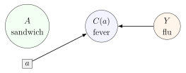
Conditioning on fever opens a path between sandwich type and influenza.

Since \(Y\) is not downstream of \(A\), there is no causal effect of sandwich on influenza. Unconditionally, \(A\) and \(Y\) may be independent. But conditioning on fever induces dependence: among people with fever, knowing the person ate chicken salad makes influenza more likely because chicken salad did not explain the fever.

Key Idea

Conditioning can create bias when the conditioned variable is a collider or a descendant of a collider.

25.4 Causal Effect among Compliers

In some randomized studies, assignment \(Z\) is randomized but treatment actually taken \(A\) is not fully controlled. Some participants comply with assignment, while others do not. A common causal target is the effect among compliers: \[\mathbb{E}\{Y(1)-Y(0)\,\vert\,A(1)=1,A(0)=0\},\] where \(A(z)\) is the treatment that would be taken under assignment \(Z=z\).

This estimand is not an ordinary ATE in the full population. It is an effect in a latent subgroup defined by joint potential treatment behaviors under two assignment levels.

25.5 Principal Stratification

Principal stratification defines subgroups using potential values of an intermediate variable. For example, in a vaccine study, one might ask for the effect of vaccination on growth among children who would have been infected without vaccination: \[\mathbb{E}\{G(1)-G(0)\,\vert\,I(0)=1\}.\] Here \(I(0)\) is infection status under no vaccination and \(G(a)\) is growth under vaccination level \(a\).

Principal strata can be scientifically appealing, but they often involve cross-world or partially latent quantities. Identification typically requires assumptions beyond standard exchangeability and positivity.

25.6 Transition from Identification to Estimation

This chapter has produced observed-data parameters for causal quantities. For example, \[\mathbb{E}\{Y(a)\} = \mathbb{E}\{\mathbb{E}(Y\,\vert\,A=a,W)\}\] and \[\mathbb{E}\{Y(a)\} = \mathbb{E}\left\{ \frac{\mathbb{1}(A=a)Y}{\mathbb{P}(A=a\,\vert\,W)} \right\}.\] These formulas do not yet tell us how to estimate the quantities in finite samples. They tell us what must be estimated: outcome regressions, propensity scores, covariate distributions, and expectations.

Estimation Notes

The next step is estimation. Once identification has converted counterfactual parameters into observed-data parameters, we can construct estimators such as plug-in G-computation estimators, IPTW estimators, and later doubly robust estimators.

Chapter 4. Basic Estimation of the Average Treatment Effect

Lecture 4.1. From Identification to Estimation

26.1 Observed Data Structure: \(O=(W,A,Y)\)

In the previous chapter, the average treatment effect was identified under consistency, conditional randomization, and positivity. Identification gave formulas involving only the observed-data distribution. Estimation begins after that step: we now have a sample and must turn the identified statistical parameter into a numerical estimate.

Throughout this chapter the observed data are \[O_i=(W_i,A_i,Y_i), \qquad i=1,\ldots,n,\] where the observations are assumed to be independent and identically distributed: \[O_1,\ldots,O_n \overset{\mathrm{iid}}{\sim}P.\] Here \(W\) is a vector of pre-treatment covariates, \(A\in\{0,1\}\) is treatment, and \(Y\) is the outcome. The phrase “pre-treatment” is important. Variables affected by treatment are not ordinary confounders for the effect of \(A\) on \(Y\) in a point-treatment analysis, because adjusting for them can block part of the causal effect or create collider bias.

Causal Assumption

The estimators in this chapter are estimators of causal effects only when the identification assumptions from Chapter 3 are scientifically credible: \[Y(a)=Y \text{ if } A=a,\qquad Y(a)\perp\!\!\!\perp A\,\vert\,W,\qquad \mathbb{P}(A=a\,\vert\,W=w)>0\] for all treatment levels \(a\) and all covariate values \(w\) in the target population. Without these assumptions, the same formulas estimate well-defined statistical parameters, but those parameters need not equal counterfactual means.

26.2 Outcome Regression \(\overline{Q}(a,w)\)

Definition 26.1 (Outcome regression). The outcome regression is the conditional mean of the observed outcome given treatment and covariates: \[\overline{Q}(a,w)=\mathbb{E}(Y\,\vert\,A=a,W=w).\]

This function answers an observed-data question: among individuals who actually received treatment level \(a\) and had covariates \(W=w\), what was the mean outcome? Under the identification assumptions, this observed subgroup mean can be used as a building block for the mean counterfactual outcome under treatment level \(a\).

For a binary outcome, \(\overline{Q}(a,w)\) is a conditional risk: \[\overline{Q}(a,w)=\mathbb{P}(Y=1\,\vert\,A=a,W=w).\] For a continuous outcome, it is a conditional average. For an ordinal or count outcome, it is still a conditional mean, although the mean may not fully summarize the whole conditional distribution.

26.3 Propensity Score \(g_a(w)\)

Definition 26.2 (Propensity score). For a binary treatment, the treatment-specific propensity score is \[g_a(w)=\mathbb{P}(A=a\,\vert\,W=w).\] The usual propensity score is \(g_1(w)=\mathbb{P}(A=1\,\vert\,W=w)\), and \(g_0(w)=1-g_1(w)\).

The propensity score describes how treatment is assigned in the observed population. It is not a causal effect. Instead, it measures the treatment probability among people with covariate value \(w\). In inverse probability weighting, individuals who received a treatment level that was unlikely for their covariates receive larger weights. These weights compensate for the unequal representation of covariate strata across treatment groups.

26.4 Plug-In Estimation

The g-computation identification formula for the counterfactual mean is \[\psi(a)=\mathbb{E}\{Y(a)\}=\mathbb{E}\{\overline{Q}(a,W)\}.\] This formula contains two features of the observed-data distribution: the conditional mean function \(\overline{Q}(a,w)\) and the marginal distribution of \(W\). A plug-in estimator replaces each unknown population quantity by an estimate from the data.

Definition 26.3 (Plug-in estimator). A plug-in estimator is obtained by writing the target parameter as a function of the observed-data distribution and then substituting empirical or model-based estimates for the unknown components of that distribution.

If \(\overline{Q}_n(a,w)\) estimates \(\overline{Q}(a,w)\), the natural g-computation plug-in estimator is \[\psi_n^{\mathrm{gcomp}}(a) = \frac{1}{n}\sum_{i=1}^n \overline{Q}_n(a,W_i).\] This expression averages predicted outcomes under treatment level \(a\) over the observed covariate distribution. The observed covariates \(W_1,\ldots,W_n\) are used as an empirical approximation to the target population distribution of \(W\).

Estimation turns the identified observed-data parameter into a sample quantity.

26.5 Estimating Counterfactual Means

There are two basic plug-in strategies emphasized in this chapter.

The first uses the outcome regression: \[\psi_n^{\mathrm{gcomp}}(a)=\frac{1}{n}\sum_{i=1}^n \overline{Q}_n(a,W_i).\] For each observed individual, we keep \(W_i\) fixed and replace the observed treatment by the hypothetical treatment value \(a\) inside the fitted outcome regression. The resulting predicted values are then averaged.

The second uses inverse probability weighting. If \(g_{n,a}(w)\) estimates \(g_a(w)=\mathbb{P}(A=a\,\vert\,W=w)\), then \[\psi_n^{\operatorname{IPTW}}(a) = \frac{1}{n}\sum_{i=1}^n \frac{\mathbb{1}(A_i=a)}{g_{n,a}(W_i)}Y_i.\] Only people who actually received treatment level \(a\) contribute to the estimate of \(\mathbb{E}\{Y(a)\}\), but their outcomes are weighted by the inverse of their estimated probability of receiving that treatment.

Key Idea

G-computation estimates counterfactual means by predicting everyone’s outcome under each treatment level. IPTW estimates counterfactual means by reweighting the people who actually received each treatment level so that, after weighting, they represent the full target population.

26.6 Estimating the ATE

The average treatment effect is \[\operatorname{ATE}=\mathbb{E}\{Y(1)\}-\mathbb{E}\{Y(0)\}=\psi(1)-\psi(0).\] The corresponding g-computation estimator is \[\widehat{\operatorname{ATE}}_{\mathrm{gcomp}} = \frac{1}{n}\sum_{i=1}^n \left\{ \overline{Q}_n(1,W_i)-\overline{Q}_n(0,W_i) \right\}.\] The corresponding IPTW estimator is \[\widehat{\operatorname{ATE}}_{\operatorname{IPTW}} = \frac{1}{n}\sum_{i=1}^n \left\{ \frac{\mathbb{1}(A_i=1)}{g_{n,1}(W_i)}Y_i - \frac{\mathbb{1}(A_i=0)}{g_{n,0}(W_i)}Y_i \right\}.\]

Estimation Notes

Basic estimation workflow for the ATE:

Choose whether to estimate the counterfactual means using the outcome regression, the propensity score, or both in a later doubly robust method.
Estimate the nuisance function required by the chosen method.
Construct \(\psi_n(1)\) and \(\psi_n(0)\) using the identified formula.
Report \(\widehat{\operatorname{ATE}}=\psi_n(1)-\psi_n(0)\).
Quantify uncertainty using an appropriate variance estimator or resampling method such as the bootstrap.

Lecture 4.2. G-Computation with Discrete Data

27.1 Empirical Mean Outcome Regression

When \(W\) takes only a small number of possible values, the most direct estimator of the outcome regression is the sample mean within each \((A,W)\) subgroup. For a fixed treatment value \(a\) and covariate value \(w\), define \[n_{aw}=\sum_{i=1}^n \mathbb{1}(A_i=a,W_i=w).\] If \(n_{aw}>0\), the empirical outcome regression is \[\overline{Q}_n(a,w) = \frac{\sum_{i=1}^n Y_i\mathbb{1}(A_i=a,W_i=w)} {\sum_{i=1}^n \mathbb{1}(A_i=a,W_i=w)}.\] This is simply the average observed outcome among people with treatment \(A=a\) and covariates \(W=w\).

For example, if \(W\) is a binary age indicator, then \(\overline{Q}_n(1,0)\) is the sample mean outcome among younger treated individuals, while \(\overline{Q}_n(0,1)\) is the sample mean outcome among older untreated individuals.

Key Idea

With low-dimensional discrete covariates, empirical g-computation is ordinary stratification. Estimate the mean outcome in each treatment-covariate stratum, then average those stratum means using the covariate distribution of the target population.

27.2 Saturated Regression Models

A saturated model has enough parameters to reproduce every subgroup mean. With binary \(A\) and binary \(W\), there are four treatment-covariate subgroups. A saturated linear mean model is \[\mathbb{E}(Y\,\vert\,A=a,W=w)=\beta_0+\beta_1 a+\beta_2 w+\beta_3 aw.\] The fitted means implied by this model are \[\begin{array}{c|cc} & A=0 & A=1\\ \hline W=0 & \beta_0 & \beta_0+\beta_1\\ W=1 & \beta_0+\beta_2 & \beta_0+\beta_1+\beta_2+\beta_3 . \end{array}\] Because there are four parameters and four subgroup means, the model can exactly match the empirical subgroup averages whenever each subgroup is observed. The interaction term \(aw\) is what makes the model saturated. Without it, the model would force the treatment contrast to be the same at both levels of \(W\) on the additive scale.

Remark 75. The word “saturated” is about flexibility relative to the chosen covariate description. If \(W\) has many categories or multiple components, a truly saturated model may require many main effects and interactions.

27.3 Estimating \(\mathbb{P}(W=w)\)

The g-computation parameter also requires the marginal distribution of \(W\): \[\psi(a)=\sum_w \overline{Q}(a,w)\mathbb{P}(W=w).\] For discrete \(W\), the empirical estimator is the sample proportion \[P_n(W=w) = \frac{1}{n}\sum_{i=1}^n \mathbb{1}(W_i=w).\] This is the fraction of the sample in covariate stratum \(w\). It estimates the covariate distribution in the target population represented by the sample.

27.4 Computing \(\mathbb{E}\{Y(1)\}\)

The g-computation estimator of \(\mathbb{E}\{Y(1)\}\) is obtained by setting \(a=1\): \[\psi_n(1) = \sum_w \overline{Q}_n(1,w)P_n(W=w).\] For binary \(W\), this becomes \[\psi_n(1) = \overline{Q}_n(1,0)P_n(W=0)+\overline{Q}_n(1,1)P_n(W=1).\] The first term is the estimated treated mean outcome among people with \(W=0\), weighted by how common \(W=0\) is in the full sample. The second term is the analogous quantity for \(W=1\).

27.5 Computing \(\mathbb{E}\{Y(0)\}\)

Similarly, \[\psi_n(0) = \sum_w \overline{Q}_n(0,w)P_n(W=w),\] and for binary \(W\), \[\psi_n(0) = \overline{Q}_n(0,0)P_n(W=0)+\overline{Q}_n(0,1)P_n(W=1).\] This estimates the mean outcome that would have been observed if everyone in the target population had received treatment level \(0\).

27.6 Computing the ATE

The estimated average treatment effect is the difference between the two estimated counterfactual means: \[\widehat{\operatorname{ATE}}_{\mathrm{gcomp}} = \psi_n(1)-\psi_n(0).\] Equivalently, \[\widehat{\operatorname{ATE}}_{\mathrm{gcomp}} = \sum_w \left\{ \overline{Q}_n(1,w)-\overline{Q}_n(0,w) \right\}P_n(W=w).\] This expression shows that empirical g-computation is a weighted average of stratum-specific treatment contrasts. The weights are not the covariate distributions inside the treated and untreated groups separately. They are the covariate distribution of the full target sample.

27.7 Equivalent Individual-Level Form

Because \(P_n(W=w)\) is the fraction of individuals whose covariates equal \(w\), the same estimator can be written as \[\psi_n(a) = \frac{1}{n}\sum_{i=1}^n \overline{Q}_n(a,W_i).\] To see this, start from the subgroup formula: \[\sum_w \overline{Q}_n(a,w)P_n(W=w) = \sum_w \overline{Q}_n(a,w) \left\{ \frac{1}{n}\sum_{i=1}^n \mathbb{1}(W_i=w) \right\}.\] Move the finite sum over observations outside: \[= \frac{1}{n}\sum_{i=1}^n \sum_w \overline{Q}_n(a,w)\mathbb{1}(W_i=w).\] For each individual \(i\), exactly one value of \(w\) equals \(W_i\), so the inner sum is \(\overline{Q}_n(a,W_i)\). Therefore, \[\sum_w \overline{Q}_n(a,w)P_n(W=w) = \frac{1}{n}\sum_{i=1}^n \overline{Q}_n(a,W_i).\]

27.8 By-Hand Example

Suppose \(W\) is binary and the sample summaries are as follows: \[\begin{array}{c|cc|c} W & \overline{Q}_n(0,W) & \overline{Q}_n(1,W) & P_n(W)\\ \hline 0 & 2.680 & 2.875 & 0.370\\ 1 & 2.222 & 2.327 & 0.630 \end{array}\] Then \[\psi_n(1)=2.875(0.370)+2.327(0.630)=2.530,\] and \[\psi_n(0)=2.680(0.370)+2.222(0.630)=2.392.\] Thus \[\widehat{\operatorname{ATE}}_{\mathrm{gcomp}}=2.530-2.392=0.138.\] The interpretation is that, after standardizing the treated and untreated subgroup means to the same covariate distribution, the estimated mean outcome is about 0.138 units higher under treatment than under no treatment.

Estimation Notes

By-hand empirical g-computation:

List all observed covariate strata \(w\).
Compute \(\overline{Q}_n(1,w)\) and \(\overline{Q}_n(0,w)\) within each stratum.
Compute \(P_n(W=w)\) for each stratum.
Form \(\psi_n(1)=\sum_w \overline{Q}_n(1,w)P_n(W=w)\).
Form \(\psi_n(0)=\sum_w \overline{Q}_n(0,w)P_n(W=w)\).
Subtract to obtain \(\widehat{\operatorname{ATE}}_{\mathrm{gcomp}}\).

Lecture 4.3. G-Computation Using Regression Models

28.1 Prediction-Based Implementation

Empirical g-computation by hand is transparent, but it becomes cumbersome when \(W\) has many components. Regression provides a systematic way to estimate \(\overline{Q}(a,w)=\mathbb{E}(Y\,\vert\,A=a,W=w)\) and then evaluate the fitted regression under counterfactual treatment values.

The generic regression-based g-computation estimator is \[\psi_n(a)=\frac{1}{n}\sum_{i=1}^n \overline{Q}_n(a,W_i),\] where \(\overline{Q}_n\) is a fitted outcome regression. The estimated ATE is \[\widehat{\operatorname{ATE}}_{\mathrm{gcomp}} = \frac{1}{n}\sum_{i=1}^n \left\{\overline{Q}_n(1,W_i)-\overline{Q}_n(0,W_i)\right\}.\]

This estimator has two conceptually distinct stages. First, estimate conditional outcome means from the observed data. Second, average predicted outcomes under treatment levels that may differ from the treatment actually observed for a given individual.

28.2 Using `predict()` with Counterfactual Treatment Values

In software, the most stable way to implement g-computation is to create two modified copies of the covariate data: \[\text{data}^{(1)}=(W_i,A_i=1)_{i=1}^n,\qquad \text{data}^{(0)}=(W_i,A_i=0)_{i=1}^n.\] The fitted outcome model is then used to predict the outcome for every row of each modified dataset.

Implementation Notes

Generic R pattern for g-computation:

# fit an outcome regression
fit_Q <- glm(Y ~ A + W, data = dat, family = gaussian())

# create treatment-specific prediction datasets
dat1 <- dat
dat1$A <- 1
dat0 <- dat
dat0$A <- 0

# predict under each treatment level
Q1 <- predict(fit_Q, newdata = dat1, type = "response")
Q0 <- predict(fit_Q, newdata = dat0, type = "response")

# estimate counterfactual means and ATE
psi1 <- mean(Q1)
psi0 <- mean(Q0)
ate  <- psi1 - psi0

The argument newdata is crucial. It asks the fitted regression to evaluate the conditional mean at covariate-treatment combinations chosen by the analyst, not only at the treatment values actually observed.

28.3 Saturated GLMs

For discrete covariates, a saturated generalized linear model can reproduce the empirical subgroup means. With binary \(A\) and binary \(W\), a saturated linear model is \[\mathbb{E}(Y\,\vert\,A=a,W=w) = \beta_0+\beta_1a+\beta_2w+\beta_3aw.\] If a Gaussian working model with identity link is fit by least squares, the predictions at the four \((a,w)\) combinations equal the four observed subgroup sample means.

For a binary outcome, a saturated logistic model can be written as \[\mathop{\mathrm{logit}}\{\mathbb{P}(Y=1\,\vert\,A=a,W=w)\} = \beta_0+\beta_1a+\beta_2w+\beta_3aw.\] Its fitted probabilities can match the empirical risks in each subgroup, provided the data do not have complete separation and each subgroup contains observations. The link function changes the parameterization, but saturation still means that no subgroup restriction is imposed beyond the chosen covariate coding.

28.4 Main-Terms GLMs

In practice, analysts often use smoother, lower-dimensional regressions. A main-terms linear outcome model is \[\overline{Q}_n(a,w)=\hat\beta_0+\hat\beta_1 a+\hat\beta_2^\top w.\] The g-computation estimator is then \[\psi_n(a) = \frac{1}{n}\sum_{i=1}^n \left(\hat\beta_0+\hat\beta_1 a+\hat\beta_2^\top W_i\right) = \hat\beta_0+\hat\beta_1 a+\hat\beta_2^\top \bar W_n,\] where \(\bar W_n=n^{-1}\sum_i W_i\). Therefore, \[\widehat{\operatorname{ATE}}_{\mathrm{gcomp}} = \psi_n(1)-\psi_n(0) = \hat\beta_1.\] This equality is a special property of the identity-link linear main-terms model. It does not hold for most other models.

If the model includes a treatment-covariate interaction, \[\overline{Q}_n(a,w)=\hat\beta_0+\hat\beta_1 a+\hat\beta_2^\top w+\hat\beta_3^\top(aw),\] then \[\widehat{\operatorname{ATE}}_{\mathrm{gcomp}} = \frac{1}{n}\sum_{i=1}^n \left(\hat\beta_1+\hat\beta_3^\top W_i\right) = \hat\beta_1+\hat\beta_3^\top \bar W_n.\] The coefficient \(\hat\beta_1\) is the estimated treatment contrast when \(W=0\), not the population-average treatment effect unless \(\bar W_n=0\) or \(\hat\beta_3=0\).

28.5 Logistic Regression G-Computation

Suppose \(Y\) is binary and we fit a main-terms logistic regression \[\overline{Q}_n(a,w) = \mathop{\mathrm{expit}}(\hat\gamma_0+\hat\gamma_1a+\hat\gamma_2^\top w).\] The g-computation estimator is \[\psi_n(1) = \frac{1}{n}\sum_{i=1}^n \mathop{\mathrm{expit}}(\hat\gamma_0+\hat\gamma_1+\hat\gamma_2^\top W_i),\] \[\psi_n(0) = \frac{1}{n}\sum_{i=1}^n \mathop{\mathrm{expit}}(\hat\gamma_0+\hat\gamma_2^\top W_i),\] and \[\widehat{\operatorname{ATE}}_{\mathrm{gcomp}} = \frac{1}{n}\sum_{i=1}^n \left[ \mathop{\mathrm{expit}}(\hat\gamma_0+\hat\gamma_1+\hat\gamma_2^\top W_i) - \mathop{\mathrm{expit}}(\hat\gamma_0+\hat\gamma_2^\top W_i) \right].\]

Implementation Notes

Logistic regression g-computation in R:

fit_Q <- glm(Y ~ A + W, data = dat, family = binomial())

dat1 <- dat
dat1$A <- 1
dat0 <- dat
dat0$A <- 0

Q1 <- predict(fit_Q, newdata = dat1, type = "response")
Q0 <- predict(fit_Q, newdata = dat0, type = "response")

psi1 <- mean(Q1)
psi0 <- mean(Q0)
ate  <- psi1 - psi0

28.6 Why Logistic Coefficients Are Not ATEs

The coefficient \(\hat\gamma_1\) in a logistic regression is a conditional log odds ratio parameter. It compares the log odds of the outcome between treatment groups at a fixed value of \(W\), assuming the model is correctly specified on the log odds scale. The ATE is a marginal risk difference: \[\mathbb{E}\{Y(1)\}-\mathbb{E}\{Y(0)\}.\] These are different objects.

There are three reasons the logistic treatment coefficient is not generally an ATE. First, it is on the log odds scale, whereas the ATE is a mean difference or risk difference. Second, it is conditional on \(W\), whereas the ATE averages over the population distribution of \(W\). Third, the expit function is nonlinear, so averaging after applying the inverse-logit is not the same as applying the inverse-logit after averaging: \[\frac{1}{n}\sum_{i=1}^n \mathop{\mathrm{expit}}(\eta_i) \neq \mathop{\mathrm{expit}}\left(\frac{1}{n}\sum_{i=1}^n \eta_i\right)\] in general.

Key Idea

For regression-based g-computation, the causal estimate is the average contrast of predicted counterfactual outcomes. Regression coefficients are intermediate nuisance quantities. They are not automatically causal effects.

Lecture 4.4. IPTW with Discrete Data

29.1 Estimating Propensity Scores by Hand

The inverse probability weighted estimator is motivated by the identification result \[\mathbb{E}\{Y(a)\} = \mathbb{E}\left\{ \frac{\mathbb{1}(A=a)}{g_a(W)}Y \right\}, \qquad g_a(W)=\mathbb{P}(A=a\,\vert\,W).\] With discrete \(W\), the propensity score can be estimated within each covariate stratum. For binary treatment, \[g_{n,1}(w) = \frac{\sum_{i=1}^n \mathbb{1}(A_i=1,W_i=w)} {\sum_{i=1}^n \mathbb{1}(W_i=w)},\] and \[g_{n,0}(w)=1-g_{n,1}(w).\] Thus \(g_{n,1}(w)\) is the sample proportion treated among individuals with \(W=w\).

If \(W\) is binary, this gives two treatment probabilities: \[g_{n,1}(0)=\frac{\#\{i:A_i=1,W_i=0\}}{\#\{i:W_i=0\}}, \qquad g_{n,1}(1)=\frac{\#\{i:A_i=1,W_i=1\}}{\#\{i:W_i=1\}}.\]

29.2 Estimating Propensity Scores Using Regression

The same quantities can be obtained from a saturated logistic regression for treatment. With binary \(W\), \[\mathbb{P}(A=1\,\vert\,W=w)=\mathop{\mathrm{expit}}(\gamma_0+\gamma_1w).\] There are two parameters and two covariate strata, so the fitted probabilities can match the empirical treatment proportions in the two strata.

Implementation Notes

Saturated propensity score model for binary \(W\):

fit_g <- glm(A ~ W, data = dat, family = binomial())

newW <- data.frame(W = c(0, 1))
g1_by_W <- predict(fit_g, newdata = newW, type = "response")
g0_by_W <- 1 - g1_by_W

For more complex discrete \(W\), a saturated treatment model requires enough terms to represent the treatment probability in every covariate stratum. When \(W\) is large or continuous, analysts usually use a lower-dimensional regression or machine learning method to smooth across similar covariate values.

29.3 Estimating the Joint Distribution

The fully discrete IPTW plug-in estimator can be written by estimating the joint distribution of \((W,A,Y)\). If \(W\), \(A\), and \(Y\) are discrete, the empirical joint probability is \[P_n(W=w,A=a,Y=y) = \frac{1}{n}\sum_{i=1}^n \mathbb{1}(W_i=w,A_i=a,Y_i=y).\] Plugging this empirical distribution and the estimated propensity score into the IPTW identification formula gives \[\psi_n(a) = \sum_{w,a',y} \frac{\mathbb{1}(a'=a)}{g_{n,a}(w)} y\,P_n(W=w,A=a',Y=y).\] The summation uses \(a'\) as a dummy treatment value to avoid confusion with the target intervention level \(a\).

29.4 Computing Inverse Probability Weights

For target treatment level \(a\), the inverse probability weight for observation \(i\) is \[\omega_i(a)=\frac{\mathbb{1}(A_i=a)}{g_{n,a}(W_i)}.\] If an individual actually received treatment level \(a\), their weight is the inverse of the estimated probability of receiving that treatment. If they did not receive treatment level \(a\), their weight is zero for estimating \(\mathbb{E}\{Y(a)\}\).

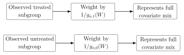
IPTW reweights each observed treatment group to represent the target population.

Extreme weights arise when \(g_{n,a}(W_i)\) is close to zero. Such observations can dominate the estimate, which is why positivity is not merely a technical detail.

29.5 Estimating \(\mathbb{E}\{Y(1)\}\), \(\mathbb{E}\{Y(0)\}\), and the ATE

Using the empirical joint distribution, the estimator simplifies to the individual-level sample average \[\psi_n(a) = \frac{1}{n}\sum_{i=1}^n \frac{\mathbb{1}(A_i=a)}{g_{n,a}(W_i)}Y_i.\] The derivation follows by substituting the empirical distribution: \[\begin{aligned} \sum_{w,a',y} &\frac{\mathbb{1}(a'=a)}{g_{n,a}(w)} y\,P_n(W=w,A=a',Y=y)\\ &= \sum_{w,a',y} \frac{\mathbb{1}(a'=a)}{g_{n,a}(w)} y\left\{ \frac{1}{n}\sum_{i=1}^n \mathbb{1}(W_i=w,A_i=a',Y_i=y) \right\}\\ &= \frac{1}{n}\sum_{i=1}^n \sum_{w,a',y} \frac{\mathbb{1}(a'=a)}{g_{n,a}(w)} y\mathbb{1}(W_i=w,A_i=a',Y_i=y)\\ &= \frac{1}{n}\sum_{i=1}^n \frac{\mathbb{1}(A_i=a)}{g_{n,a}(W_i)}Y_i. \end{aligned}\] Therefore, \[\psi_n(1) = \frac{1}{n}\sum_{i=1}^n \frac{\mathbb{1}(A_i=1)}{g_{n,1}(W_i)}Y_i,\] \[\psi_n(0) = \frac{1}{n}\sum_{i=1}^n \frac{\mathbb{1}(A_i=0)}{g_{n,0}(W_i)}Y_i,\] and \[\widehat{\operatorname{ATE}}_{\operatorname{IPTW}}=\psi_n(1)-\psi_n(0).\]

Using the same binary-\(W\) summaries from empirical g-computation, suppose \[g_{n,1}(0)=0.476,\qquad g_{n,0}(0)=0.524,\] and \[g_{n,1}(1)=0.486,\qquad g_{n,0}(1)=0.514.\] The IPTW calculation weights each observed outcome by the inverse probability of the treatment actually received. When the propensity scores are empirical stratum proportions, the weighted treated mean reproduces the same standardized quantity as empirical g-computation: \[\psi_n(1)=2.530,\qquad \psi_n(0)=2.392,\] and therefore \[\widehat{\operatorname{ATE}}_{\operatorname{IPTW}}=2.530-2.392=0.138.\] This numerical equality is a special property of the fully empirical discrete estimator. It should not be expected once lower-dimensional regression smoothing is used for \(\overline{Q}_n\) or \(g_n\).

Implementation Notes

Regression-based IPTW in R:

fit_g <- glm(A ~ W, data = dat, family = binomial())

g1 <- predict(fit_g, type = "response")
g0 <- 1 - g1

psi1 <- mean((dat$A == 1) / g1 * dat$Y)
psi0 <- mean((dat$A == 0) / g0 * dat$Y)
ate  <- psi1 - psi0

Estimation Notes

By-hand IPTW with discrete data:

Estimate \(g_{n,1}(w)\) and \(g_{n,0}(w)\) in every covariate stratum.
For each observation, compute \(\omega_i(1)=\mathbb{1}(A_i=1)/g_{n,1}(W_i)\) and \(\omega_i(0)=\mathbb{1}(A_i=0)/g_{n,0}(W_i)\).
Compute \(\psi_n(1)=n^{-1}\sum_i \omega_i(1)Y_i\).
Compute \(\psi_n(0)=n^{-1}\sum_i \omega_i(0)Y_i\).
Subtract to estimate the ATE.

Lecture 4.5. Comparing G-Computation and IPTW

30.1 When Empirical G-Computation and IPTW Coincide

In the fully discrete setting, if both nuisance functions are estimated by empirical subgroup proportions and means, empirical g-computation and empirical IPTW give the same point estimate. This equality is not a general property of all g-computation and IPTW estimators. It is a special algebraic feature of saturated discrete estimation.

Proposition 30.1 (Equivalence under empirical discrete estimation). Suppose \(W\) is discrete, every relevant \((A=a,W=w)\) cell is nonempty, and \[\overline{Q}_n(a,w) = \frac{\sum_{i=1}^nY_i\mathbb{1}(A_i=a,W_i=w)} {\sum_{i=1}^n\mathbb{1}(A_i=a,W_i=w)}, \qquad g_{n,a}(w) = \frac{\sum_{i=1}^n\mathbb{1}(A_i=a,W_i=w)} {\sum_{i=1}^n\mathbb{1}(W_i=w)}.\] Then \[\frac{1}{n}\sum_{i=1}^n \overline{Q}_n(a,W_i) = \frac{1}{n}\sum_{i=1}^n \frac{\mathbb{1}(A_i=a)}{g_{n,a}(W_i)}Y_i.\]

Proof. Let \(n_w=\sum_i\mathbb{1}(W_i=w)\) and \(n_{aw}=\sum_i\mathbb{1}(A_i=a,W_i=w)\). The g-computation estimator can be written as \[\sum_w \overline{Q}_n(a,w)\frac{n_w}{n}.\] Substituting the empirical subgroup mean, \[\sum_w \left\{ \frac{\sum_iY_i\mathbb{1}(A_i=a,W_i=w)}{n_{aw}} \right\} \frac{n_w}{n}.\] Substituting \(g_{n,a}(w)=n_{aw}/n_w\) gives \[\frac{1}{n}\sum_w \sum_i Y_i\mathbb{1}(A_i=a,W_i=w) \frac{1}{g_{n,a}(w)}.\] For each observation \(i\), only the term with \(w=W_i\) contributes, so the expression equals \[\frac{1}{n}\sum_{i=1}^n \frac{\mathbb{1}(A_i=a)}{g_{n,a}(W_i)}Y_i,\] which is the IPTW estimator. ◻

30.2 Why the Equivalence Is Special

The proof above uses two facts. First, \(\overline{Q}_n(a,w)\) is the empirical mean in exactly the same strata used to estimate \(g_{n,a}(w)\). Second, the empirical covariate distribution gives each stratum weight \(n_w/n\). If either nuisance function is estimated by a model that smooths across strata, the exact cancellation in the proof usually disappears.

Key Idea

G-computation and IPTW are equivalent as identification formulas under the causal assumptions. Their finite-sample estimators need not be equal, because the fitted outcome regression and fitted propensity score can approximate different parts of the observed-data distribution in different ways.

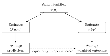
The two methods estimate the same causal parameter through different nuisance functions.

30.3 High-Dimensional Discrete Covariates

Empirical stratification becomes fragile when \(W\) has many discrete components. If \(W=(W_1,\ldots,W_p)\) and each \(W_j\) is binary, then \(W\) can take \(2^p\) possible values. Even moderate \(p\) can create many sparse or empty strata.

Sparse strata create two problems. For g-computation, \(\overline{Q}_n(a,w)\) is unstable when only a few observations have \(A=a\) and \(W=w\), and undefined when no such observation exists. For IPTW, \(g_{n,a}(w)\) is unstable when treatment counts are small, and the weights \(1/g_{n,a}(w)\) can become extremely large.

30.4 Continuous Covariates

If \(W\) contains a continuous component, exact empirical stratification usually fails. In a continuous distribution, the probability that two individuals have exactly the same covariate vector is often zero. Then the subgroup \[\{i:W_i=w\}\] may contain only one observation or none, making empirical subgroup means unusable.

This is not a conceptual problem for the estimand. The counterfactual mean \[\psi(a)=\mathbb{E}\{\overline{Q}(a,W)\}\] is still well-defined. The difficulty is statistical: we must estimate the smooth conditional mean or treatment probability from finite data.

30.5 Need for Regression Smoothing

Regression smoothing borrows information across similar covariate values. Instead of estimating a separate mean for every exact \(w\), a model might assume \[\overline{Q}(a,w)=\beta_0+\beta_1a+\beta_2^\top w\] or \[g_1(w)=\mathop{\mathrm{expit}}(\alpha_0+\alpha_1^\top w).\] These restrictions reduce variance, but they introduce the possibility of model misspecification. A simple main-terms model may be too rigid if the true outcome regression has nonlinearities or treatment-covariate interactions.

The central estimation tradeoff is therefore: \[\text{less smoothing} \Rightarrow \text{lower modeling bias but higher variance},\] \[\text{more smoothing} \Rightarrow \text{lower variance but higher risk of bias}.\]

30.6 Variance and Instability

IPTW estimators are especially sensitive to near-violations of positivity. If \(g_{n,1}(W_i)=0.02\), then a treated individual receives weight \(50\). A small number of such observations can strongly influence the weighted mean.

G-computation can also be unstable or biased, but the failure mode is different. A poor outcome regression may extrapolate into covariate-treatment combinations with little support. For example, if very old individuals are almost never treated, then \(\overline{Q}_n(1,w)\) for very old \(w\) is largely determined by model assumptions rather than direct data.

Estimation Notes

Practical comparison:

Empirical g-computation and empirical IPTW coincide in low-dimensional discrete settings with nonempty cells.
Regression-based g-computation and regression-based IPTW usually differ.
G-computation relies most directly on the quality of the outcome regression.
IPTW relies most directly on the quality of the propensity score and on stable positivity.
Large weights, empty cells, and extrapolation are diagnostic signs that the data may not contain enough information for the desired causal contrast without strong modeling assumptions.

Lecture 4.6. G-Computation and IPTW in R

31.1 Data Preparation

The R implementations of g-computation and IPTW are most reliable when the data are prepared so that the notation matches the analysis. The dataset should contain one row per individual and variables corresponding to \(W\), \(A\), and \(Y\): \[O_i=(W_i,A_i,Y_i).\] Treatment should be coded consistently, often as \(A=1\) for treated and \(A=0\) for untreated. Binary outcomes should also be coded as \(0/1\) when logistic regression is used.

Implementation Notes

Example setup:

# dat has one row per individual
# A: binary treatment, coded 0/1
# Y: outcome
# W1, W2: pre-treatment covariates

dat <- dat[complete.cases(dat[, c("Y", "A", "W1", "W2")]), ]
dat$A <- as.numeric(dat$A == 1)
dat$Y <- as.numeric(dat$Y)

Dropping observations with missing data is simple but not always appropriate. If missingness is related to treatment, outcome, or covariates, complete-case analysis can change the target population or introduce bias. Later chapters treat missing data more carefully.

31.2 Fitting Outcome Regressions

For g-computation, the nuisance function is \[\overline{Q}(a,w)=\mathbb{E}(Y\,\vert\,A=a,W=w).\] The fitted outcome regression should include treatment and the confounders required for identification. It may also include interactions or nonlinear terms if scientifically or statistically warranted.

Implementation Notes

Outcome regression examples:

# Continuous outcome, identity link
fit_Q_linear <- glm(Y ~ A + W1 + W2, data = dat, family = gaussian())

# Binary outcome, logistic link
fit_Q_logistic <- glm(Y ~ A + W1 + W2, data = dat, family = binomial())

# Interaction model allowing treatment effect heterogeneity by W1
fit_Q_interact <- glm(Y ~ A * W1 + W2, data = dat, family = binomial())

The fitted object is not itself the causal estimate. It is an estimate of a nuisance function used to compute predicted counterfactual outcomes.

31.3 Fitting Propensity Score Models

For IPTW, the nuisance function is \[g_1(w)=\mathbb{P}(A=1\,\vert\,W=w).\] Because \(A\) is binary, logistic regression is a common starting point: \[\mathop{\mathrm{logit}}\{g_1(w)\}=\alpha_0+\alpha^\top w.\]

Implementation Notes

Propensity score model:

fit_g <- glm(A ~ W1 + W2, data = dat, family = binomial())

g1 <- predict(fit_g, type = "response")
g0 <- 1 - g1

After fitting the propensity score, inspect whether predicted probabilities are close to zero or one. Very small \(g_1(W_i)\) among treated individuals or very small \(g_0(W_i)\) among untreated individuals lead to large IPTW weights.

31.4 Prediction Workflows

The g-computation prediction workflow constructs the two estimated counterfactual means by changing only the treatment variable:

\[\psi_n(1)=\frac{1}{n}\sum_{i=1}^n\overline{Q}_n(1,W_i), \qquad \psi_n(0)=\frac{1}{n}\sum_{i=1}^n\overline{Q}_n(0,W_i).\]

Implementation Notes

G-computation prediction workflow:

dat1 <- dat
dat1$A <- 1

dat0 <- dat
dat0$A <- 0

Q1 <- predict(fit_Q_logistic, newdata = dat1, type = "response")
Q0 <- predict(fit_Q_logistic, newdata = dat0, type = "response")

psi1_gcomp <- mean(Q1)
psi0_gcomp <- mean(Q0)
ate_gcomp  <- psi1_gcomp - psi0_gcomp

For IPTW, no treatment-specific prediction datasets are required. The estimator uses the observed treatment and observed outcome: \[\psi_n^{\operatorname{IPTW}}(a)= \frac{1}{n}\sum_{i=1}^n \frac{\mathbb{1}(A_i=a)}{g_{n,a}(W_i)}Y_i.\]

Implementation Notes

IPTW workflow:

A <- dat$A
Y <- dat$Y

psi1_iptw <- mean((A == 1) / g1 * Y)
psi0_iptw <- mean((A == 0) / g0 * Y)
ate_iptw  <- psi1_iptw - psi0_iptw

31.5 Treatment-Specific Datasets

Treatment-specific datasets are useful because they make the estimand visible in the code. The dataset dat1 represents the empirical covariate distribution with everyone assigned \(A=1\); dat0 represents the same empirical covariate distribution with everyone assigned \(A=0\).

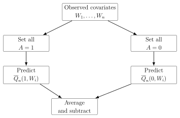
Treatment-specific datasets implement g-computation predictions.

This workflow should not be confused with changing the observed data. The original outcomes remain the data used to fit the outcome model. The modified datasets are only prediction grids used to evaluate the fitted conditional mean.

31.6 Practical Implementation Patterns

It is often helpful to wrap estimators in functions. This makes bootstrap inference straightforward and reduces the chance of accidentally using variables from the wrong dataset.

Implementation Notes

Reusable g-computation function:

get_gcomp <- function(input_data) {
  fit_Q <- glm(Y ~ A + W1 + W2, data = input_data, family = binomial())

  data1 <- input_data
  data1$A <- 1
  data0 <- input_data
  data0$A <- 0

  Q1 <- predict(fit_Q, newdata = data1, type = "response")
  Q0 <- predict(fit_Q, newdata = data0, type = "response")

  c(psi0 = mean(Q0), psi1 = mean(Q1), ate = mean(Q1) - mean(Q0))
}

Implementation Notes

Reusable IPTW function:

get_iptw <- function(input_data) {
  fit_g <- glm(A ~ W1 + W2, data = input_data, family = binomial())

  g1 <- predict(fit_g, type = "response")
  g0 <- 1 - g1

  A <- input_data$A
  Y <- input_data$Y

  psi1 <- mean((A == 1) / g1 * Y)
  psi0 <- mean((A == 0) / g0 * Y)

  c(psi0 = psi0, psi1 = psi1, ate = psi1 - psi0)
}

Estimation Notes

Implementation checks:

Confirm that \(A\), \(Y\), and all covariates are coded as intended.
For g-computation, confirm that newdata contains the same covariate names and factor levels as the model-fitting dataset.
For IPTW, inspect summaries of \(g_1\), \(g_0\), and the resulting weights.
Keep the estimation function self-contained so that resampling methods refit all nuisance functions inside each resampled dataset.

Lecture 4.7. Bootstrap Inference

32.1 Why Variance Formulas Are Complex

Point estimates alone are not enough. A causal analysis should also report uncertainty: standard errors, confidence intervals, and sometimes hypothesis tests. For g-computation and IPTW, uncertainty comes from several sources at once.

For g-computation, the estimator \[\psi_n^{\mathrm{gcomp}}(a) = \frac{1}{n}\sum_{i=1}^n \overline{Q}_n(a,W_i)\] depends on the empirical distribution of \(W\) and on the fitted outcome regression \(\overline{Q}_n\). For IPTW, the estimator \[\psi_n^{\operatorname{IPTW}}(a) = \frac{1}{n}\sum_{i=1}^n \frac{\mathbb{1}(A_i=a)}{g_{n,a}(W_i)}Y_i\] depends on the empirical distribution of \((W,A,Y)\) and on the fitted propensity score \(g_{n,a}\). Treating \(\overline{Q}_n\) or \(g_n\) as fixed after fitting usually understates uncertainty because it ignores the fact that the nuisance functions were estimated from the same data.

Key Idea

The standard error must reflect the entire estimation procedure, not only the final sample average. When nuisance functions are fit from data, their variability is part of the variability of the causal effect estimator.

32.2 Nonparametric Bootstrap

The nonparametric bootstrap approximates repeated sampling by resampling the observed data. Let \(\psi_n\) denote an estimator of a counterfactual mean or ATE. A bootstrap replicate is constructed as follows:

Sample \(n\) rows from the original dataset with replacement.
Refit all nuisance models in this bootstrap dataset.
Recompute the complete estimator in the bootstrap dataset.

Repeating these steps \(M\) times gives bootstrap estimates \[\psi_n^{\#,1},\psi_n^{\#,2},\ldots,\psi_n^{\#,M}.\] The symbol \(\#\) is used here to distinguish bootstrap estimates from the original estimate \(\psi_n\).

Each bootstrap replicate repeats the full estimation procedure.

32.3 Bootstrap Confidence Intervals

A percentile bootstrap confidence interval uses quantiles of the bootstrap estimates. For a nominal 95% interval, let \(\psi_n^\#(0.025)\) and \(\psi_n^\#(0.975)\) be the empirical 2.5th and 97.5th percentiles of \(\psi_n^{\#,1},\ldots,\psi_n^{\#,M}\). The interval is \[\left[ \psi_n^\#(0.025),\ \psi_n^\#(0.975) \right].\] This interval is easy to compute and often adequate for introductory analyses, but it can perform poorly in small samples, with highly skewed estimators, or when the estimator is irregular.

32.4 Bootstrap Standard Errors

The bootstrap standard error is the sample standard deviation of the bootstrap estimates: \[\hat\sigma^\# = \left[ \frac{1}{M-1}\sum_{m=1}^M \left(\psi_n^{\#,m}-\bar\psi_n^\#\right)^2 \right]^{1/2},\] where \[\bar\psi_n^\#=\frac{1}{M}\sum_{m=1}^M \psi_n^{\#,m}.\] This standard error can be reported directly or used in Wald-style confidence intervals of the form \[\psi_n\pm 1.96\,\hat\sigma^\#.\]

32.5 Wald-Style p-Values

For testing \[H_0:\psi=0 \qquad\text{versus}\qquad H_1:\psi\neq 0,\] a Wald-style test statistic is \[Z=\frac{\psi_n}{\hat\sigma^\#}.\] Using the standard normal approximation, the two-sided p-value is \[p=2\left\{1-\Phi(|Z|)\right\},\] where \(\Phi\) is the cumulative distribution function of the standard normal distribution.

This p-value inherits the assumptions of the large-sample approximation and the bootstrap standard error. It should be interpreted as a statistical summary, not as a measure of whether the causal assumptions are true.

32.6 Bootstrap for G-Computation

The key rule is that the outcome regression must be refit in every bootstrap sample. If the fitted model from the original data is reused, the bootstrap will miss an important component of uncertainty.

Implementation Notes

Bootstrap for g-computation:

get_gcomp <- function(input_data) {
  fit_Q <- glm(Y ~ A + W1 + W2, data = input_data, family = binomial())

  data1 <- input_data
  data1$A <- 1
  data0 <- input_data
  data0$A <- 0

  Q1 <- predict(fit_Q, newdata = data1, type = "response")
  Q0 <- predict(fit_Q, newdata = data0, type = "response")

  psi1 <- mean(Q1)
  psi0 <- mean(Q0)
  c(psi0 = psi0, psi1 = psi1, ate = psi1 - psi0)
}

set.seed(1234)
M <- 1000
n <- nrow(dat)

boot_ate <- numeric(M)

for (m in seq_len(M)) {
  boot_ids <- sample(seq_len(n), size = n, replace = TRUE)
  boot_dat <- dat[boot_ids, ]
  boot_ate[m] <- get_gcomp(boot_dat)["ate"]
}

est <- get_gcomp(dat)["ate"]
se_boot <- sd(boot_ate)
ci_boot <- quantile(boot_ate, probs = c(0.025, 0.975))
p_value <- 2 * pnorm(-abs(est / se_boot))

The same bootstrap draws can be used to compute confidence intervals for \(\psi(0)\), \(\psi(1)\), and the ATE if the function returns all three quantities.

32.7 Bootstrap for IPTW

For IPTW, the propensity score model must be refit in every bootstrap sample. The weights in each bootstrap replicate should be computed from the bootstrap-fitted propensity scores, not from the original fitted propensity scores.

Implementation Notes

Bootstrap for IPTW:

get_iptw <- function(input_data) {
  fit_g <- glm(A ~ W1 + W2, data = input_data, family = binomial())

  g1 <- predict(fit_g, type = "response")
  g0 <- 1 - g1

  A <- input_data$A
  Y <- input_data$Y

  psi1 <- mean((A == 1) / g1 * Y)
  psi0 <- mean((A == 0) / g0 * Y)
  c(psi0 = psi0, psi1 = psi1, ate = psi1 - psi0)
}

set.seed(1234)
M <- 1000
n <- nrow(dat)

boot_ate <- numeric(M)

for (m in seq_len(M)) {
  boot_ids <- sample(seq_len(n), size = n, replace = TRUE)
  boot_dat <- dat[boot_ids, ]
  boot_ate[m] <- get_iptw(boot_dat)["ate"]
}

est <- get_iptw(dat)["ate"]
se_boot <- sd(boot_ate)
ci_boot <- quantile(boot_ate, probs = c(0.025, 0.975))
p_value <- 2 * pnorm(-abs(est / se_boot))

Estimation Notes

Bootstrap checklist:

Resample rows, not individual variables independently.
Refit every nuisance model inside each bootstrap sample.
Recompute the entire estimator from the resampled data.
Use enough bootstrap replicates for stable quantiles; \(M=1000\) is a common minimum for routine work.
Inspect failed model fits, separation warnings, and extreme weights, because these are informative signs of instability.

Chapter 5. Super Learning

Lecture 5.1. Why Flexible Regression Is Needed

33.1 Limitations of Empirical Moment Estimators

The g-computation and IPTW estimators from Chapter 4 require nuisance functions: \[\overline{Q}(a,w)=\mathbb{E}(Y\,\vert\,A=a,W=w), \qquad g_a(w)=\mathbb{P}(A=a\,\vert\,W=w).\] When \(W\) is low-dimensional and discrete, these functions can be estimated by empirical subgroup means and proportions. For example, \[\overline{Q}_n(a,w)= \frac{\sum_{i=1}^nY_i\mathbb{1}(A_i=a,W_i=w)} {\sum_{i=1}^n\mathbb{1}(A_i=a,W_i=w)}\] is reasonable if there are enough observations in every treatment-covariate stratum.

This approach fails as soon as the number of strata is large relative to the sample size. If \(W\) contains ten binary variables, there are \(2^{10}=1024\) possible covariate patterns before treatment is even considered. Many cells will be empty, and many nonempty cells will contain too few observations to estimate a stable conditional mean. The same problem affects the propensity score: a stratum with only one treated and no untreated individuals cannot support both \(g_1(w)\) and \(g_0(w)\) empirically.

Key Idea

Empirical moment estimators are transparent but local. They use only observations with exactly the same covariate values. That is attractive in small discrete examples, but it becomes unstable or undefined when covariates are high-dimensional or continuous.

33.2 Continuous Covariates

Continuous covariates make exact stratification especially problematic. Suppose \(W\) is body mass index or age measured in years and decimals. In a continuous distribution, the probability that two people have exactly the same value of \(W\) is often close to zero. Then the empirical subgroup \[\{i:W_i=w\}\] is empty for most values \(w\) and may contain only one individual at observed values.

The target function \(\overline{Q}(a,w)\) is still meaningful. The question \[\mathbb{E}(Y\,\vert\,A=1,W=-3.5)\] asks for the average outcome among treated individuals with covariate value \(-3.5\). The problem is not conceptual; it is statistical. A finite sample does not contain many people with exactly that covariate value, so we need a method that uses information from nearby or otherwise similar covariate values.

33.3 Borrowing Information Across Covariate Values

To estimate \(\overline{Q}(a,w)\) at a particular \(w\), we must decide which observations are informative about that point. Observations with covariates very close to \(w\) are usually more relevant than observations far away from \(w\), but using only the closest observations can produce a noisy estimate.

The same issue appears for the propensity score. To estimate \[g_1(w)=\mathbb{P}(A=1\,\vert\,W=w),\] we need to learn how treatment probabilities vary with \(W\). If we use only people with exactly \(W=w\), the estimate is unstable. If we use everyone equally, the estimate may ignore important differences in treatment assignment across covariates.

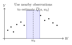
Flexible regression borrows information across covariate values.

33.4 Regression as Smoothing

Regression is a formal way to borrow information. A regression estimator smooths the observed outcomes across covariate values in order to estimate a conditional mean function. The amount and shape of smoothing depend on the method.

A linear regression with \[\overline{Q}(a,w)=\beta_0+\beta_1a+\beta_2w\] borrows information very aggressively. The model assumes that a one-unit change in \(W\) has the same additive association with \(Y\) everywhere. If this is true, the method can be efficient. If it is false, the method may be biased.

A kernel regression borrows information locally. It estimates \(\overline{Q}(a,w)\) using observations whose covariates are close to \(w\). A regression tree borrows information within leaves of a fitted tree. A random forest averages many such trees. A generalized additive model borrows information through smooth functions of predictors. Each method embodies a different answer to the same question: which observations should inform the prediction at a given covariate value, and how much should they count?

33.5 Why Model Choice Matters for Causal Estimators

In causal inference, nuisance regression quality matters because causal estimators are functions of these regressions. For g-computation, \[\widehat{\operatorname{ATE}}_{\mathrm{gcomp}} = \frac{1}{n}\sum_{i=1}^n \left\{\overline{Q}_n(1,W_i)-\overline{Q}_n(0,W_i)\right\}.\] If \(\overline{Q}_n\) is biased in regions of the covariate space that are common in the target population, the ATE estimate can be biased.

For IPTW, \[\widehat{\operatorname{ATE}}_{\operatorname{IPTW}} = \frac{1}{n}\sum_{i=1}^n \left\{ \frac{\mathbb{1}(A_i=1)}{g_{n,1}(W_i)}Y_i - \frac{\mathbb{1}(A_i=0)}{g_{n,0}(W_i)}Y_i \right\}.\] If \(g_n\) is poorly estimated, the weights can be wrong, unstable, or both.

Causal Assumption

Flexible regression does not replace causal assumptions. Consistency, conditional randomization, and positivity are still required to interpret the resulting statistical estimates causally. Super Learning helps estimate observed-data nuisance functions; it does not make unmeasured confounding disappear.

Estimation Notes

The practical objective in this chapter is to estimate nuisance functions well enough for causal estimation. We therefore need a principled way to compare candidate regression estimators before using them inside g-computation, IPTW, or later doubly robust estimators.

Lecture 5.2. Bias–Variance Tradeoff

34.1 Low Bias vs High Variance

Bias and variance describe two different ways an estimator can perform poorly. Suppose the target regression function is \[Q_0(a,w)=\mathbb{E}(Y\,\vert\,A=a,W=w),\] and \(\overline{Q}_n(a,w)\) is an estimator computed from a sample. At a fixed point \((a,w)\), the bias is the difference between the average value of the estimator across repeated samples and the truth: \[\mathop{\mathrm{Bias}}\{\overline{Q}_n(a,w)\} = \mathbb{E}\{\overline{Q}_n(a,w)\}-Q_0(a,w).\] The variance describes how much \(\overline{Q}_n(a,w)\) changes from sample to sample: \[\mathop{\mathrm{Var}}\{\overline{Q}_n(a,w)\} = \mathbb{E}\left[ \left\{\overline{Q}_n(a,w)-\mathbb{E}\{\overline{Q}_n(a,w)\}\right\}^2 \right].\]

An estimator can have low bias but high variance. For example, an estimator that uses only people with covariates extremely close to \(w\) may target the local conditional mean accurately, but because it uses very few observations, its estimate can fluctuate substantially across samples.

34.2 High Bias vs Low Variance

An estimator can also have high bias but low variance. A simple linear regression may use the full sample and therefore produce stable estimates. But if the true regression function is strongly nonlinear, the fitted line may systematically miss the truth.

Key Idea

Bias is systematic error from using a method that is too rigid or otherwise wrong. Variance is random error from using a method that is too sensitive to the particular sample. Good prediction requires balancing both.

34.3 Kernel Regression Intuition

Kernel regression provides a concrete picture of the bias-variance tradeoff. Consider estimating \(\mathbb{E}(Y\,\vert\,A=1,W=w_0)\). A simple local estimator is the uniform-kernel estimator \[\overline{Q}_{n,h}(1,w_0) = \frac{\sum_{i=1}^nY_i\mathbb{1}(A_i=1)\mathbb{1}(|W_i-w_0|\le h/2)} {\sum_{i=1}^n\mathbb{1}(A_i=1)\mathbb{1}(|W_i-w_0|\le h/2)}.\] The tuning parameter \(h>0\) is the bandwidth. The estimator averages outcomes among treated individuals whose \(W\) values fall inside a window of width \(h\) centered at \(w_0\).

If \(h\) is small, the estimator uses only very similar people. That reduces bias when the regression function changes with \(W\), but it increases variance because the estimate is based on fewer observations. If \(h\) is large, the estimator uses more people. That reduces variance but may introduce bias by averaging over people who are not very similar to \(w_0\).

34.4 Bandwidth Choice

Bandwidth choice is a model selection problem. There is no universally best bandwidth because the optimal choice depends on the unknown smoothness of the true regression function and on the sample size. A very smooth true function can tolerate a larger bandwidth. A highly curved true function requires a smaller bandwidth to avoid oversmoothing.

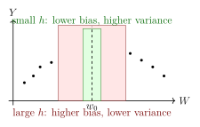
The bandwidth controls how much information is borrowed across covariate values.

34.5 Parametric vs Semiparametric vs Nonparametric Methods

Regression methods differ in how strongly they restrict the true regression function.

Definition 34.1 (Parametric method). A parametric regression method assumes that the regression function belongs to a finite-dimensional family, such as \[\overline{Q}(a,w)=\beta_0+\beta_1a+\beta_2^\top w.\]

Parametric methods can have low variance because they impose strong structure, but they can have high bias if the structure is wrong.

Definition 34.2 (Semiparametric method). A semiparametric method combines finite-dimensional components with flexible components. For example, \[\overline{Q}(a,w)=\beta_0+\beta_1a+f(w)\] leaves the function \(f\) unspecified or only weakly restricted.

Definition 34.3 (Nonparametric method). A nonparametric method allows the regression function to become increasingly flexible as the sample size grows. Examples include kernel regression, random forests, neural networks, and certain spline or tree-based methods.

The labels are less important than the practical consequence: different methods borrow information in different ways and therefore occupy different points in the bias-variance tradeoff.

34.6 Unknown True Regression Function

If the true regression function were known to be linear, a linear model would be a natural choice. If the true function were known to have sharp interactions, a more adaptive method would be needed. In practice, the true function is unknown.

This uncertainty is the motivation for Super Learning. Rather than choosing one regression method because it is familiar, we pre-specify a library of plausible candidate methods and use cross-validated risk to compare them.

Estimation Notes

For causal estimation, model choice is not merely a prediction issue. Bias in \(\overline{Q}_n\) can bias g-computation; instability in \(g_n\) can destabilize IPTW. The next lectures develop a risk-based framework for choosing or combining nuisance function estimators.

Lecture 5.3. Risk and Loss Functions

35.1 Prediction Loss

To compare regression estimators, we need a numerical score. A loss function measures how bad a prediction is for one observation. If \(\overline{Q}_n\) predicts the outcome using \(A\) and \(W\), then a loss function assigns a number \[L(\overline{Q}_n)(W,A,Y)\] to the prediction-observation pair. Smaller loss means better prediction.

The choice of loss should match the regression target. If the target is the conditional mean of a continuous outcome, squared-error loss is natural. If the target is the conditional probability of a binary outcome, negative log-likelihood loss is natural.

35.2 Squared-Error Loss

For a continuous or mean-valued outcome regression, squared-error loss is \[L(\overline{Q}_n)(w,a,y) = \{y-\overline{Q}_n(a,w)\}^2.\] This loss heavily penalizes large prediction errors because the error is squared. It is the standard loss for estimating conditional means.

35.3 Negative Log-Likelihood Loss

For a binary outcome \(Y\in\{0,1\}\), an outcome regression estimates \[\overline{Q}(a,w)=\mathbb{P}(Y=1\,\vert\,A=a,W=w).\] If \(\overline{Q}_n(a,w)\) is a predicted probability, the Bernoulli likelihood contribution is \[\overline{Q}_n(a,w)^y\{1-\overline{Q}_n(a,w)\}^{1-y}.\] The negative log-likelihood loss is \[L(\overline{Q}_n)(w,a,y) = -\log\left[ \overline{Q}_n(a,w)^y\{1-\overline{Q}_n(a,w)\}^{1-y} \right].\] Equivalently, \[L(\overline{Q}_n)(w,a,y) = -y\log\{\overline{Q}_n(a,w)\} -(1-y)\log\{1-\overline{Q}_n(a,w)\}.\] This loss rewards assigning high probability to the outcome that actually occurred and strongly penalizes confident but wrong predictions.

35.4 Risk as Average Loss

Definition 35.1 (Risk). The risk of a regression estimator \(\overline{Q}_n\) under loss \(L\) is the expected loss under the true observed-data distribution: \[R(\overline{Q}_n)=\mathbb{E}\left\{L(\overline{Q}_n)(W,A,Y)\right\}.\] For discrete \((W,A,Y)\), \[R(\overline{Q}_n) = \sum_{w,a,y} L(\overline{Q}_n)(w,a,y)\mathbb{P}(W=w,A=a,Y=y).\]

Risk is the average prediction error we would expect if the fitted regression were evaluated on new observations from the same population. The best estimator is the one with the smallest risk, provided the loss function is appropriate for the target.

35.5 Valid Loss Functions

Definition 35.2 (Valid loss function). A loss function is valid for a regression target \(\overline{Q}\) if the true regression function minimizes the population risk: \[\overline{Q}\in \mathop{\mathrm{arg\,min}}_Q R(Q).\]

This definition formalizes the idea that the scoring rule should reward estimators for getting close to the true target. Squared-error loss is valid for conditional means. Bernoulli negative log-likelihood loss is valid for conditional probabilities.

35.6 Why the True Regression Minimizes Risk

We now show why squared-error loss targets the conditional mean. Let \[\overline{Q}(A,W)=\mathbb{E}(Y\,\vert\,A,W)\] be the true outcome regression, and let \(Q(A,W)\) be any candidate prediction function. The squared-error risk is \[R(Q)=\mathbb{E}\left[\{Y-Q(A,W)\}^2\right].\] Add and subtract the true regression: \[Y-Q(A,W) = \{Y-\overline{Q}(A,W)\}+\{\overline{Q}(A,W)-Q(A,W)\}.\] Squaring and taking expectations gives \[\begin{aligned} R(Q) &= \mathbb{E}\left[ \{Y-\overline{Q}(A,W)\}^2 \right]\\ &\quad+ 2\mathbb{E}\left[ \{Y-\overline{Q}(A,W)\}\{\overline{Q}(A,W)-Q(A,W)\} \right]\\ &\quad+ \mathbb{E}\left[ \{\overline{Q}(A,W)-Q(A,W)\}^2 \right]. \end{aligned}\] The middle term is zero. To see this, use iterated expectation: \[\begin{aligned} &\mathbb{E}\left[ \{Y-\overline{Q}(A,W)\}\{\overline{Q}(A,W)-Q(A,W)\} \right]\\ &= \mathbb{E}\left[ \{\overline{Q}(A,W)-Q(A,W)\} \mathbb{E}\{Y-\overline{Q}(A,W)\,\vert\,A,W\} \right]. \end{aligned}\] But \[\mathbb{E}\{Y-\overline{Q}(A,W)\,\vert\,A,W\} = \mathbb{E}(Y\,\vert\,A,W)-\overline{Q}(A,W)=0.\] Therefore, \[R(Q) = \mathbb{E}\left[ \{Y-\overline{Q}(A,W)\}^2 \right] + \mathbb{E}\left[ \{\overline{Q}(A,W)-Q(A,W)\}^2 \right].\] The first term does not depend on \(Q\). The second term is nonnegative and equals zero only when \(Q(A,W)=\overline{Q}(A,W)\) with probability one. Thus the true conditional mean minimizes squared-error risk.

Key Idea

Risk is useful because an appropriate loss function turns regression estimation into a well-defined competition: the estimator with lower risk is closer to the true regression target in the sense encoded by the loss.

35.7 Risk Decomposition into Noise, Bias, and Variance

Risk also clarifies the bias-variance tradeoff. Under squared-error loss, \[R(\overline{Q}_n) = \mathbb{E}\left[ \{Y-\overline{Q}(A,W)\}^2 \right] + \mathbb{E}\left[ \{\overline{Q}(A,W)-\overline{Q}_n(A,W)\}^2 \right].\] The first term is irreducible noise: even the true conditional mean cannot predict the individual outcome perfectly.

Now decompose the second term. Add and subtract the repeated-sampling expectation \(\mathbb{E}\{\overline{Q}_n(A,W)\}\): \[\overline{Q}(A,W)-\overline{Q}_n(A,W) = \left[\overline{Q}(A,W)-\mathbb{E}\{\overline{Q}_n(A,W)\}\right] + \left[\mathbb{E}\{\overline{Q}_n(A,W)\}-\overline{Q}_n(A,W)\right].\] After squaring and taking expectations, the cross-term is zero by the definition of the expectation of \(\overline{Q}_n\). Thus \[\begin{aligned} \mathbb{E}\left[ \{\overline{Q}(A,W)-\overline{Q}_n(A,W)\}^2 \right] &= \mathbb{E}\left[ \{\overline{Q}(A,W)-\mathbb{E}\{\overline{Q}_n(A,W)\}\}^2 \right] \\ &\quad+ \mathbb{E}\left[ \{\mathbb{E}\{\overline{Q}_n(A,W)\}-\overline{Q}_n(A,W)\}^2 \right]. \end{aligned}\] The first term is squared bias and the second is variance. Therefore squared-error risk can be viewed as \[\text{risk} = \text{noise}+\text{bias}^2+\text{variance}.\]

Estimation Notes

Cross-validation will estimate risk using validation observations that were not used to fit the candidate regression. This matters because empirical risk on the training sample can reward overfitting and give an overly optimistic score.

Lecture 5.4. Cross-Validated Risk Assessment

36.1 The Problem with Empirical Risk

The population risk \[R(\overline{Q}_n)=\mathbb{E}\{L(\overline{Q}_n)(W,A,Y)\}\] cannot be computed directly because the true distribution of \((W,A,Y)\) is unknown. A tempting estimate is the empirical risk on the same data used to fit \(\overline{Q}_n\): \[R_n(\overline{Q}_n) = \frac{1}{n}\sum_{i=1}^n L(\overline{Q}_n)(W_i,A_i,Y_i).\] For squared-error loss, this is \[R_n(\overline{Q}_n) = \frac{1}{n}\sum_{i=1}^n \{Y_i-\overline{Q}_n(A_i,W_i)\}^2.\]

The problem is that \(\overline{Q}_n\) was trained to fit these same observations. A flexible method can make training errors very small without learning a relationship that generalizes to new data.

36.2 Overfitting

Overfitting occurs when an estimator captures idiosyncratic noise in the training data instead of the stable signal in the population. A twentieth-degree polynomial may thread through the observed data points and have very low training error, while a third-degree polynomial may better approximate the true regression function on new observations.

Training error is therefore often optimistic. It can also select the wrong method: the method with the lowest empirical risk on the training data may have worse risk in the population.

Key Idea

To evaluate prediction performance fairly, predictions should be tested on observations that were not used to fit the prediction rule.

36.3 Training and Validation Samples

Cross-validation mimics external validation by splitting the observed sample into two roles:

a training sample used to fit the regression estimator;
a validation sample used only to evaluate prediction loss.

If \(\overline{Q}_{n,T}\) is fit using training set \(T\) and evaluated on validation set \(V\), the validation risk estimate is \[R_{n,V}(\overline{Q}_{n,T}) = \frac{1}{|V|}\sum_{i\in V} L(\overline{Q}_{n,T})(W_i,A_i,Y_i).\] Because the validation observations were not used to fit \(\overline{Q}_{n,T}\), this estimate is a more honest measure of out-of-sample predictive performance.

36.4 V-Fold Cross-Validation

In \(V\)-fold cross-validation, the data are partitioned into \(V\) approximately equal folds. Let \(\mathcal V_v\) denote the validation indices in fold \(v\), and let \(\mathcal T_v\) be the remaining training indices. For each fold:

fit the candidate estimator on \(\mathcal T_v\);
predict outcomes for observations in \(\mathcal V_v\);
compute the average validation loss in \(\mathcal V_v\).

The cross-validated risk is the average validation loss over folds: \[R_{CV,n}(\overline{Q}_n) = \frac{1}{V}\sum_{v=1}^V \left[ \frac{1}{|\mathcal V_v|} \sum_{i\in\mathcal V_v} L(\overline{Q}_{n,v})(W_i,A_i,Y_i) \right],\] where \(\overline{Q}_{n,v}\) is the estimator fit without the validation fold \(\mathcal V_v\). When folds are equal size, this is equivalent to the average loss across all out-of-fold predictions.

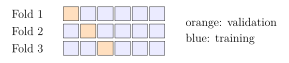
In V-fold cross-validation, each fold is used once for validation.

36.5 Choosing the Number of Folds

The number of folds controls a practical tradeoff.

With a larger \(V\), each training set is closer in size to the full dataset. This can be helpful in small samples or with flexible algorithms that need many observations to train well. Leave-one-out cross-validation is the extreme case \(V=n\).

With a smaller \(V\), each validation fold is larger. This can make validation risk estimates more stable, especially when outcomes are rare or highly skewed. Smaller \(V\) is also computationally cheaper because fewer models are fit.

Common choices include \(V=5\) and \(V=10\). The choice should be made before looking at which algorithms win.

36.6 Cross-Validated Risk as External-Data Mimicry

The ideal way to evaluate a regression estimator would be to fit it in the study sample and test it in a new independent sample from the same population. Such data are rarely available. Cross-validation approximates this ideal by repeatedly creating temporary training and validation samples from the observed data.

This matters for causal inference because nuisance functions are often selected before being inserted into causal effect estimators. Cross-validated risk gives a pre-specified, objective criterion for choosing among candidate outcome regressions or propensity score models.

Estimation Notes

V-fold cross-validation workflow:

Split the sample into \(V\) folds.
For each candidate regression estimator and each fold, fit the estimator on the training folds.
Predict on the held-out fold.
Compute validation loss.
Average validation loss over folds.
Prefer candidates with lower cross-validated risk.

Lecture 5.5. Candidate Estimator Selection

37.1 Pre-Specifying the Candidate Library

A candidate library is a set of regression algorithms chosen before looking at which one gives the desired causal result. For outcome regression, the library might contain linear regression, logistic regression, generalized additive models, random forests, lasso, regression trees, splines, and neural networks. For propensity score estimation, the same broad idea applies, but the outcome being predicted is treatment \(A\) rather than outcome \(Y\).

Definition 37.1 (Candidate library). A candidate library is a pre-specified collection \[\mathcal L=\{\mathcal A_1,\ldots,\mathcal A_K\}\] of regression algorithms. When algorithm \(\mathcal A_k\) is trained on the observed data, it produces a fitted regression estimator \(\overline{Q}_{n,k}\) or \(g_{n,k}\).

The library should be broad enough to include methods with different bias-variance profiles. A useful library often contains both simple stable methods and flexible adaptive methods. The simple methods protect against overfitting in small samples; the flexible methods protect against bias when the true regression is complex.

37.2 Comparing Regressions Using Cross-Validated Risk

For each candidate algorithm \(k\), compute its cross-validated risk: \[R_{CV,n}(\overline{Q}_{n,k}) = \frac{1}{V}\sum_{v=1}^V \frac{1}{|\mathcal V_v|} \sum_{i\in\mathcal V_v} L(\overline{Q}_{n,k,v})(W_i,A_i,Y_i),\] where \(\overline{Q}_{n,k,v}\) is algorithm \(k\) fit on the training data excluding validation fold \(\mathcal V_v\).

The candidate with the smallest cross-validated risk is selected: \[k_{CV} = \mathop{\mathrm{arg\,min}}_{k\in\{1,\ldots,K\}} R_{CV,n}(\overline{Q}_{n,k}).\] The selected algorithm is then refit on the full dataset to produce the final nuisance function estimate.

37.3 Discrete Super Learner

Definition 37.2 (Discrete Super Learner). The discrete Super Learner is the cross-validation selector that chooses the single candidate algorithm with the lowest cross-validated risk and then refits that algorithm on the full sample.

The word “discrete” means that the final estimator is one member of the candidate library, not a weighted combination. If the library contains \(K\) algorithms, the discrete Super Learner chooses one of those \(K\) algorithms.

Estimation Notes

Discrete Super Learner for an outcome regression:

Pre-specify candidate algorithms \(\mathcal A_1,\ldots,\mathcal A_K\).
Choose a valid loss function for \(\overline{Q}\), such as squared-error loss or negative log-likelihood loss.
Compute cross-validated risk for each candidate.
Select the candidate with the smallest cross-validated risk.
Refit the selected candidate on the full sample.
Use the resulting \(\overline{Q}_n\) inside the causal estimator.

37.4 Avoiding Post-Hoc Model Checking

Traditional regression workflows often involve fitting a model, checking residual plots or diagnostic tables, adding or removing terms, and refitting. This can be useful for scientific exploration, but it creates problems for confirmatory estimation and inference if the final model is chosen after seeing the data.

The issue is not that diagnostics are bad. The issue is that ordinary standard errors and confidence intervals usually treat the final model as if it had been chosen in advance. They do not account for the uncertainty introduced by trying many models and selecting one.

Super Learning addresses this by moving model choice into a pre-specified algorithm. If one would consider a main-terms model, an interaction model, a spline model, and a random forest after inspecting diagnostics, those options can be placed in the library in advance. Cross-validated risk then supplies the selection rule.

Key Idea

The analysis plan should specify the library, loss function, cross-validation scheme, and selection rule before examining which candidate gives the most favorable causal estimate.

37.5 Using Cross-Validation for Outcome Regression and Propensity Score Estimation

The same framework applies to the two central nuisance functions: \[\overline{Q}(a,w)=\mathbb{E}(Y\,\vert\,A=a,W=w), \qquad g_1(w)=\mathbb{P}(A=1\,\vert\,W=w).\] For outcome regression, the validation loss compares predicted outcomes with observed outcomes. For propensity score estimation, the validation loss compares predicted treatment probabilities with observed treatment values.

For a binary treatment, a common propensity-score loss is the Bernoulli negative log-likelihood: \[L(g_n)(w,a) = -a\log\{g_n(w)\}-(1-a)\log\{1-g_n(w)\}.\] This loss is minimized by the true conditional treatment probability \(\mathbb{P}(A=1\,\vert\,W=w)\).

It is common for different algorithms to perform best for different nuisance functions. A highly flexible method might predict the outcome well but estimate the propensity score poorly, or vice versa. Therefore, the outcome regression library and propensity score library should be evaluated separately, with losses appropriate to each target.

Implementation Notes

Conceptual R workflow:

# Outcome regression library:
# compare algorithms by cross-validated loss for predicting Y from A and W.

# Propensity score library:
# compare algorithms by cross-validated loss for predicting A from W.

# The selected outcome algorithm and selected propensity algorithm
# need not be the same.

Lecture 5.6. Super Learner Ensembles

38.1 Weighted Combinations of Estimators

The discrete Super Learner chooses one candidate algorithm. But different algorithms may capture different features of the data. A regression tree may capture threshold effects, a generalized additive model may capture smooth nonlinearities, and a lasso model may be stable in moderately high dimensions. Instead of choosing exactly one, we can combine them.

Let \(\overline{Q}_{n,1},\ldots,\overline{Q}_{n,K}\) be fitted candidate outcome regressions. A weighted ensemble has the form \[\overline{Q}_{n,\omega}(a,w) = \sum_{k=1}^K \omega_k \overline{Q}_{n,k}(a,w),\] where \(\omega=(\omega_1,\ldots,\omega_K)\) is a vector of weights.

38.2 Convex Combinations

Super Learner commonly uses convex combinations: \[\omega_k\ge 0,\qquad \sum_{k=1}^K\omega_k=1.\] The set of all such weights is the simplex \[\Delta_K=\left\{\omega\in\mathbb{R}^K:\omega_k\ge 0,\ \sum_{k=1}^K\omega_k=1\right\}.\]

Convex combinations have a simple interpretation. If \(\omega_3=0.70\) and \(\omega_5=0.30\), the ensemble prediction is 70% from algorithm 3 and 30% from algorithm 5. Algorithms with weight zero do not contribute to the final prediction.

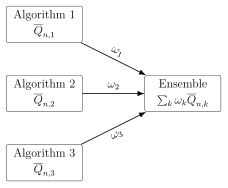
A Super Learner ensemble combines candidate predictions using learned weights.

38.3 Choosing Weights by Cross-Validated Risk Minimization

The Super Learner chooses \(\omega\) to minimize cross-validated risk. For each fold \(v\), each candidate algorithm is trained on the training folds and predicts the validation fold. For a proposed weight vector \(\omega\), the ensemble prediction in the validation fold is \[\overline{Q}_{n,\omega,v}(a,w) = \sum_{k=1}^K\omega_k\overline{Q}_{n,k,v}(a,w).\] The cross-validated risk of the ensemble is \[R_{CV,n}(\omega) = \frac{1}{V}\sum_{v=1}^V \frac{1}{|\mathcal V_v|} \sum_{i\in\mathcal V_v} L(\overline{Q}_{n,\omega,v})(W_i,A_i,Y_i).\] The selected weights are \[\omega_{CV} = \mathop{\mathrm{arg\,min}}_{\omega\in\Delta_K}R_{CV,n}(\omega).\] After the weights are selected, each candidate algorithm is refit on the full dataset, and the final Super Learner is \[\overline{Q}_{n,SL}(a,w) = \sum_{k=1}^K\omega_{CV,k}\overline{Q}_{n,k}^{\mathrm{full}}(a,w).\]

38.4 Oracle Inequalities

The theoretical appeal of Super Learner comes from oracle inequalities. An oracle is an imaginary procedure that knows the true risks of all candidates and chooses the best one. The analyst cannot implement the oracle because true risk depends on the unknown data-generating distribution.

An oracle inequality states, under regularity conditions, that the cross-validation selector or ensemble performs nearly as well as the oracle, up to a term that becomes small as sample size grows. A simplified version of the message is \[\text{risk of Super Learner} \le \text{risk of oracle choice} + \text{small remainder}.\] The remainder depends on sample size and on the size of the candidate library. This supports the practical strategy of including a diverse pre-specified library rather than trying to guess a single correct model.

Key Idea

The oracle is the best procedure in the chosen library for the data-generating distribution. Super Learner uses cross-validation to approximate that oracle without knowing the truth.

38.5 Model Stacking

Combining candidate predictions is often called stacking. The idea is to treat the out-of-fold predictions from the candidate algorithms as inputs to a second-stage learner, sometimes called the metalearner. In the convex Super Learner, the metalearner is a constrained regression that finds nonnegative weights summing to one.

Stacking differs from ordinary model averaging based on subjective preference. The weights are chosen to minimize a pre-specified cross-validated loss. This makes the ensemble a fully specified estimator rather than a post-hoc compromise among models.

38.6 Super Learner vs Single Best Algorithm

The discrete Super Learner is guaranteed to choose one candidate. The ensemble Super Learner can choose one candidate by putting all weight on it, but it can also combine multiple candidates when that lowers cross-validated risk. Thus the ensemble contains the discrete choice as a special case.

Estimation Notes

Ensemble Super Learner workflow:

Pre-specify candidate algorithms and a valid loss function.
Generate out-of-fold predictions for every algorithm.
Choose convex weights minimizing cross-validated risk.
Refit all candidate algorithms on the full dataset.
Combine full-data predictions using the selected weights.
Use the resulting nuisance function estimate inside the causal estimator.

Lecture 5.7. Practical Interpretation of Super Learner Results

39.1 Candidate Algorithms

A Super Learner analysis should report the candidate library. The library is part of the estimator. Two analyses with different libraries are using different statistical procedures, even if both are called Super Learner.

Common candidate algorithms include:

generalized linear models;
models with interactions or polynomial terms;
penalized regressions such as lasso and ridge;
generalized additive models;
multivariate adaptive regression splines;
regression trees and random forests;
gradient boosting;
Bayesian additive regression trees;
support vector machines;
neural networks;
simple empirical or intercept-only benchmarks.

The library should include algorithms with different levels of flexibility. It is often useful to include simple benchmark models because they can perform well when the sample is small or the signal is simple.

39.2 Cross-Validated Risk Tables

Super Learner output often includes a table of cross-validated risks. For squared-error loss, lower risk means lower estimated out-of-sample mean squared error. For negative log-likelihood loss, lower risk means better predicted probabilities.

A risk table might have the following conceptual form: \[\begin{array}{lcc} \toprule \text{Algorithm} & \text{CV risk for }\overline{Q}& \text{CV risk for }g\\ \midrule \text{GLM} & 1.000 & 1.000\\ \text{GAM} & 0.994 & 0.987\\ \text{Random forest} & 0.997 & 0.989\\ \text{BART} & 0.988 & 4.462\\ \text{Super Learner} & 0.986 & 0.983\\ \bottomrule \end{array}\] Risks are sometimes reported relative to a reference method, such as GLM. A relative risk below 1 means the algorithm had lower cross-validated risk than the reference. A relative risk above 1 means it performed worse by the chosen loss.

39.3 Super Learner Weights

The ensemble weights describe how the final prediction function is assembled: \[\overline{Q}_{n,SL}(a,w)=\sum_{k=1}^K\omega_k\overline{Q}_{n,k}(a,w).\] A large weight means that an algorithm contributes substantially to the final ensemble prediction. A zero weight means that the algorithm did not improve the ensemble risk given the other algorithms in the library.

Weights should not be interpreted as posterior probabilities that a model is true. A Super Learner library is not a list of mutually exclusive scientific models. It is a collection of prediction algorithms. The weights are chosen for predictive performance under a loss function, not for causal interpretation.

39.4 Why Zero Weights Are Common

Zero weights are common because many algorithms make similar predictions. If two algorithms are highly correlated, the ensemble may need only one of them. An algorithm can also receive zero weight because it predicts poorly, because it is redundant with better algorithms, or because adding it would increase validation risk.

Zero weight does not necessarily mean an algorithm is useless in all datasets. It means that, in this dataset and this library, the cross-validated metalearner did not find it helpful for reducing the chosen risk.

Key Idea

Super Learner weights are performance weights, not truth weights. They summarize how candidate predictions were combined to minimize cross-validated loss.

39.5 Outcome Regression vs Propensity Score Performance

The same algorithm can perform differently for \(\overline{Q}\) and \(g\). The outcome regression predicts \(Y\) from \((A,W)\), while the propensity score predicts \(A\) from \(W\). These are different statistical tasks.

For example, a flexible tree-based method might capture nonlinear outcome patterns well but produce unstable propensity scores near zero or one. A generalized additive model might predict treatment assignment well because the treatment mechanism is smooth, while offering little improvement for a noisy outcome.

This distinction is important for causal estimators. In g-computation, the outcome regression is the central nuisance function. In IPTW, the propensity score is central. In doubly robust estimators introduced later, both nuisance functions matter, and their estimation quality can affect bias, variance, and confidence interval behavior.

39.6 Reporting Model Libraries and Sensitivity Analyses

Transparent reporting should include:

the candidate algorithms;
important tuning parameter grids;
the loss function;
the number of cross-validation folds;
whether candidates used screening or preprocessing;
the cross-validated risks;
the selected discrete learner or ensemble weights;
any convergence failures or algorithms removed before analysis.

Sensitivity analyses are useful because Super Learner performance depends on the library. A narrow library cannot choose a method that was not included. Analysts should examine whether conclusions change when the library is expanded, when highly unstable algorithms are removed, or when alternative reasonable losses are used.

Implementation Notes

Practical reporting template:

Outcome regression:
  Loss: squared-error or negative log-likelihood
  Folds: V-fold cross-validation
  Library: GLM, GAM, lasso, random forest, ...
  Selected/weighted algorithms: report CV risks and weights

Propensity score:
  Loss: Bernoulli negative log-likelihood
  Folds: V-fold cross-validation
  Library: GLM, GAM, lasso, random forest, ...
  Diagnostics: predicted probabilities and weight summaries

Estimation Notes

When Super Learner is used inside a causal analysis, it should be described as part of the estimator of the causal parameter. Report the causal assumptions separately from the regression performance. Good cross-validated prediction does not verify exchangeability, consistency, or positivity.

Chapter 6. Super Learning Lab

Lecture 6.1. Software Setup and Simulated Data

40.1 Required R Packages

This chapter is a computational lab for the ideas developed in Chapter 5. The goal is to see how cross-validated risk minimization and Super Learner ensembles are implemented in practice. The examples use simulated data so that the true treatment mechanism and true outcome regression are known.

The main package is SuperLearner. Several other packages are often useful because they supply candidate algorithms or optimization routines. A typical setup is:

Implementation Notes

pkgs <- c("SuperLearner", "quadprog", "nloptr", "MASS",
          "ggplot2", "nnls")

installed_packages <- row.names(installed.packages())

for (p in pkgs) {
  if (!(p %in% installed_packages)) {
    install.packages(p)
  }
  library(p, character.only = TRUE)
}

The packages quadprog, nloptr, and nnls are optimization tools used by some Super Learner metalearners. The package MASS supplies regression utilities, and ggplot2 is useful for plotting. Additional candidate algorithms may require additional packages.

40.2 Loading `SuperLearner`

After installation, the package can be loaded with:

Implementation Notes

library(SuperLearner)

The package provides two kinds of functions:

user-facing functions such as SuperLearner() and CV.SuperLearner();
wrapper functions, for example SL.glm and SL.mean; these tell the package how to fit candidate algorithms.

To view available built-in learners and screeners:

Implementation Notes

listWrappers(what = "SL")
listWrappers(what = "screen")

40.3 Simulated Covariates

We simulate \(n\) independent observations with two covariates: \[W_1\sim N(0,1), \qquad W_2\sim \operatorname{Uniform}(0,1).\] These covariates are deliberately simple, but they are rich enough to illustrate interactions and nonlinear candidate regressions.

Implementation Notes

set.seed(212)

n <- 500
W1 <- rnorm(n = n)
W2 <- runif(n = n)

40.4 Simulated Treatment Mechanism

Treatment is binary. The true propensity score is \[g_1(W)=\mathbb{P}(A=1\,\vert\,W) = \mathop{\mathrm{expit}}(-1+W_1-W_2+2W_1W_2).\] This treatment mechanism includes an interaction between \(W_1\) and \(W_2\). A main terms logistic regression for \(A\) on \(W_1\) and \(W_2\) is therefore misspecified.

Implementation Notes

g1W <- plogis(-1 + W1 - W2 + 2 * W1 * W2)
A <- rbinom(n = n, size = 1, prob = g1W)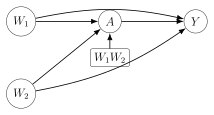

The simulated data have covariate-dependent treatment and outcome mechanisms.

40.5 Simulated Outcome Regression

The true outcome regression is linear: \[\overline{Q}(A,W)=\mathbb{E}(Y\,\vert\,A,W)=W_1-W_2+A.\] The observed outcome is generated by adding independent normal noise: \[Y=\overline{Q}(A,W)+\varepsilon,\qquad \varepsilon\sim N(0,1).\]

Implementation Notes

QAW <- W1 - W2 + A
Y <- QAW + rnorm(n = n)

full_data <- data.frame(W1 = W1, W2 = W2, A = A, Y = Y)

Because the true \(\overline{Q}\) is known, we can check whether flexible methods behave sensibly. However, in real applications the true regression function is unknown. The point of the lab is to practice methods that are useful precisely because the truth is not known.

40.6 Reproducibility with Seeds

Simulation, cross-validation splits, and some machine learning algorithms involve randomness. A random seed makes the analysis reproducible:

Implementation Notes

set.seed(212)

Using a seed does not make the result less random in a statistical sense. It fixes the particular random draw so that another analyst running the same code obtains the same simulated data, folds, and fitted results.

Key Idea

In a lab setting, seeds make examples reproducible. In a scientific analysis, they also make computational results auditable: the same data and same code should lead to the same reported estimates.

Lecture 6.2. Manual Cross-Validation

41.1 Full-Data Risk vs Cross-Validated Risk

Before calling SuperLearner(), it is useful to implement cross-validation by hand. This makes clear what the package automates.

Consider two candidate estimators for the outcome regression \(\overline{Q}(A,W)\): \[\overline{Q}_{n,1}: \text{ main-terms linear regression},\] \[\overline{Q}_{n,2}: \text{ a more flexible regression with quadratic and interaction terms}.\] The mean squared-error risk of a fitted estimator \(Q\) is \[R(Q)=\mathbb{E}\left[\{Y-Q(A,W)\}^2\right].\] The naive full-data empirical risk is \[R_n(Q_n)=\frac{1}{n}\sum_{i=1}^n\{Y_i-Q_n(A_i,W_i)\}^2.\] This quantity can be too optimistic because the same observations are used both to fit the regression and to evaluate its error.

Implementation Notes

Q1_fit <- glm(Y ~ W1 + W2 + A, data = full_data)
Q1n <- as.numeric(predict(Q1_fit))
risk_Q1_full <- mean((Y - Q1n)^2)

Q2_fit <- glm(Y ~ I(W1^2) + I(W2^2) + W1 * W2 + W1 * A + W2 * A,
              data = full_data)
Q2n <- as.numeric(predict(Q2_fit))
risk_Q2_full <- mean((Y - Q2n)^2)

41.2 Two-Fold Splitting

Two-fold cross-validation splits the data into two validation sets. Each fold is used once for validation and once as part of the training data. With two folds, the training set for fold 1 is fold 2, and the training set for fold 2 is fold 1.

Implementation Notes

split <- c(rep(1, n / 2), rep(2, n / 2))

split1 <- subset(full_data, split == 1)
split2 <- subset(full_data, split == 2)

In real analyses, folds are usually randomized rather than assigning the first half to one fold and the second half to another. For teaching, a deterministic split makes the logic easier to see.

41.3 Training Regressions

For \(\overline{Q}_{n,1}\), fit the main-terms model on split 1 and validate on split 2:

Implementation Notes

Q1_fit_split1 <- glm(Y ~ W1 + W2 + A, data = split1)
Q1n_split2 <- predict(Q1_fit_split1, newdata = split2)
risk_Q1_split2 <- mean((split2$Y - Q1n_split2)^2)

Then reverse the roles:

Implementation Notes

Q1_fit_split2 <- glm(Y ~ W1 + W2 + A, data = split2)
Q1n_split1 <- predict(Q1_fit_split2, newdata = split1)
risk_Q1_split1 <- mean((split1$Y - Q1n_split1)^2)

41.4 Validation Predictions

The essential rule is that validation predictions must be made using a model that did not train on the validation observations. For observation \(i\) in validation fold \(v\), the prediction has the form \[\overline{Q}_{n,v}(A_i,W_i),\] where \(\overline{Q}_{n,v}\) was fit using the training observations outside fold \(v\).

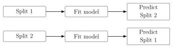
Two-fold cross-validation swaps training and validation roles.

41.5 Mean Squared-Error Risk

The two-fold cross-validated risk estimate is the average of the two fold-specific validation risks: \[R_{CV,n}(\overline{Q}_{n,1}) = \frac{1}{2}\left\{ R_{n,1}(\overline{Q}_{n,1,2})+ R_{n,2}(\overline{Q}_{n,1,1}) \right\}.\] In code:

Implementation Notes

cv_risk_Q1 <- (risk_Q1_split1 + risk_Q1_split2) / 2

For the flexible model, repeat the same process:

Implementation Notes

Q2_formula <- Y ~ I(W1^2) + I(W2^2) + W1 * W2 + W1 * A + W2 * A

Q2_fit_split1 <- glm(Q2_formula, data = split1)
Q2n_split2 <- predict(Q2_fit_split1, newdata = split2)
risk_Q2_split2 <- mean((split2$Y - Q2n_split2)^2)

Q2_fit_split2 <- glm(Q2_formula, data = split2)
Q2n_split1 <- predict(Q2_fit_split2, newdata = split1)
risk_Q2_split1 <- mean((split1$Y - Q2n_split1)^2)

cv_risk_Q2 <- (risk_Q2_split1 + risk_Q2_split2) / 2

41.6 Comparing Simple and Flexible Regressions

The candidate with lower cross-validated risk has better estimated out-of-sample prediction performance under the chosen loss. A flexible model can have lower training risk but higher cross-validated risk if it overfits. Conversely, a simple model can win when the true signal is simple or when the sample size is limited.

Key Idea

Cross-validation evaluates how well a regression predicts observations it did not use for training. This is why cross-validated risk is a better guide for selecting nuisance regressions than full-data training error.

Lecture 6.3. Manual Ensemble Construction

42.1 Ensemble Prediction Functions

An ensemble combines predictions from multiple fitted regressions. With two candidate outcome regressions \(\overline{Q}_{n,1}\) and \(\overline{Q}_{n,2}\), a convex ensemble is \[\overline{Q}_{n,\omega}(a,w) = \omega \overline{Q}_{n,1}(a,w)+(1-\omega)\overline{Q}_{n,2}(a,w), \qquad 0\le \omega\le 1.\] The weight \(\omega\) controls how much the ensemble uses the first candidate. If \(\omega=1\), the ensemble is \(\overline{Q}_{n,1}\). If \(\omega=0\), the ensemble is \(\overline{Q}_{n,2}\).

42.2 Weighted Averages of Candidate Predictions

The following function takes two fitted glm objects, obtains predictions from each, and returns their weighted average:

Implementation Notes

ensemble_predict <- function(Q1_fit, Q2_fit, newdata,
                             Q1_weight, Q2_weight = 1 - Q1_weight) {
  stopifnot(abs(1 - Q1_weight - Q2_weight) < 1e-5)

  Q1n <- predict(Q1_fit, newdata = newdata)
  Q2n <- predict(Q2_fit, newdata = newdata)

  ensemble_prediction <- Q1_weight * Q1n + Q2_weight * Q2n
  as.numeric(ensemble_prediction)
}

For one new observation, this function computes \[\omega \hat y_1+(1-\omega)\hat y_2.\] For many observations, it computes the same formula row by row.

42.3 Weight Grids

With two candidates, a simple way to search over possible ensembles is to create a grid of weights:

Implementation Notes

weight_sequence <- seq(from = 0, to = 1, length.out = 500)

Each value in weight_sequence defines a different candidate ensemble. The grid is only an approximation to the continuum \([0,1]\), but it is sufficient for illustrating the idea. With many candidates, the weight vector lies in a higher dimensional simplex, and numerical optimization methods are used instead of a simple grid.

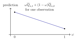
With two learners, ensemble predictions vary linearly with the weight.

42.4 Cross-Validated Risk Across Weights

For each weight, compute out-of-fold ensemble predictions and evaluate mean squared-error loss. For a fixed \(\omega\), the two-fold estimate is \[R_{CV,n}(\omega) = \frac{1}{2} \left[ \frac{1}{n_1}\sum_{i\in \mathcal V_1} \{Y_i-\overline{Q}_{n,\omega,2}(A_i,W_i)\}^2 + \frac{1}{n_2}\sum_{i\in \mathcal V_2} \{Y_i-\overline{Q}_{n,\omega,1}(A_i,W_i)\}^2 \right],\] where \(\overline{Q}_{n,\omega,2}\) is the ensemble built from models trained in split 2 and validated in split 1, and \(\overline{Q}_{n,\omega,1}\) is the analogous ensemble trained in split 1 and validated in split 2.

Implementation Notes

cv_risks <- rep(NA_real_, length(weight_sequence))

for (i in seq_along(weight_sequence)) {
  w <- weight_sequence[i]

  pred_split2 <- ensemble_predict(Q1_fit_split1, Q2_fit_split1,
                                  newdata = split2,
                                  Q1_weight = w)
  risk_split2 <- mean((split2$Y - pred_split2)^2)

  pred_split1 <- ensemble_predict(Q1_fit_split2, Q2_fit_split2,
                                  newdata = split1,
                                  Q1_weight = w)
  risk_split1 <- mean((split1$Y - pred_split1)^2)

  cv_risks[i] <- (risk_split1 + risk_split2) / 2
}

42.5 Selecting Optimal Ensemble Weights

The Super Learner weight is the value with the smallest cross-validated risk: \[\omega_{CV}=\mathop{\mathrm{arg\,min}}_{\omega\in[0,1]}R_{CV,n}(\omega).\] On a grid, this is computed by:

Implementation Notes

min_idx <- which.min(cv_risks)
omega_hat <- weight_sequence[min_idx]
min_cv_risk <- cv_risks[min_idx]

After the weight is selected, the candidate regressions are typically refit on the full dataset. The final ensemble prediction function is \[\overline{Q}_{n,SL}(a,w) = \omega_{CV}\overline{Q}_{n,1}^{\mathrm{full}}(a,w) + (1-\omega_{CV})\overline{Q}_{n,2}^{\mathrm{full}}(a,w).\]

Key Idea

Manual ensemble construction has two layers of learning. First, each candidate regression learns from training data. Second, the ensemble learns weights by comparing out-of-fold predictions.

Estimation Notes

When there are more than two candidates, Super Learner chooses weights \(\omega_1,\ldots,\omega_K\) satisfying \(\omega_k\ge 0\) and \(\sum_k\omega_k=1\). Specialized optimization routines find the cross-validated risk minimizer over this simplex more efficiently than a grid search.

Lecture 6.4. Basic Calls to `SuperLearner`

43.1 Main Arguments: `Y`, `X`, `SL.library`, `family`, `method`, `cvControl`

The function SuperLearner() automates the cross-validation and ensemble construction described in the previous lectures. Its most important arguments are:

Y: the outcome to be predicted;
X: a data frame or matrix of predictors;
SL.library: candidate algorithms;
family: the outcome family, commonly gaussian() or binomial();
method: the metalearner and loss used to choose weights;
cvControl: options controlling the internal cross-validation.

For outcome regression, Y is the observed outcome and X contains \((A,W)\). For propensity score estimation, Y is the treatment \(A\) and X contains \(W\).

Implementation Notes

set.seed(123)

sl_fit1 <- SuperLearner(
  Y = Y,
  X = data.frame(W1 = W1, W2 = W2, A = A),
  SL.library = c("SL.glm", "SL.mean"),
  family = gaussian(),
  method = "method.CC_LS",
  cvControl = list(V = 2),
  verbose = FALSE
)

43.2 Continuous vs Binary Outcomes

For a continuous outcome regression, use family = gaussian() and a loss such as squared-error loss. A common metalearner is method.CC_LS, a convex combination chosen to minimize least-squares loss.

For a binary outcome or binary treatment mechanism, use family = binomial(). For predicted probabilities, a natural loss is negative log-likelihood. A useful metalearner is method.CC_nloglik.

Implementation Notes

# Outcome regression for continuous Y
fit_Q <- SuperLearner(Y = Y,
                      X = data.frame(A = A, W1 = W1, W2 = W2),
                      SL.library = c("SL.glm", "SL.mean"),
                      family = gaussian(),
                      method = "method.CC_LS")

# Propensity score for binary A
fit_g <- SuperLearner(Y = A,
                      X = data.frame(W1 = W1, W2 = W2),
                      SL.library = c("SL.glm", "SL.mean"),
                      family = binomial(),
                      method = "method.CC_nloglik")

43.3 Interpreting Printed Output

Printing a SuperLearner object shows the call, the cross-validated risk of each candidate, and the final ensemble coefficients. A typical table has columns: \[\text{Risk},\qquad \text{Coef}.\] The risk column describes candidate performance under the chosen cross-validated loss. The coefficient column gives the ensemble weight assigned to each candidate.

43.4 Risk

The reported risk is not the full-data training error. It is an internal cross-validated risk estimate for each candidate algorithm. For Gaussian outcomes with method.CC_LS, this risk is mean squared prediction error. For binomial outcomes with method.CC_nloglik, it is negative log-likelihood risk.

Risk values are comparable only when they use the same outcome and same loss. A mean squared-error risk for \(Y\) should not be numerically compared with a negative-log-likelihood risk for \(A\).

43.5 Coefficients

The coefficients are the estimated ensemble weights. If a candidate has coefficient zero, it does not contribute to the final Super Learner prediction. This does not mean the candidate is scientifically impossible or universally poor; it means that, given the other candidates and the selected loss, the metalearner did not need that candidate to reduce cross-validated risk.

Key Idea

The risk table scores individual algorithms. The coefficients describe the ensemble. An algorithm can have mediocre individual risk but still receive weight if its predictions complement the predictions of other learners.

43.6 Super Learner Predictions

The object returned by SuperLearner() contains fitted predictions for the observed rows:

Implementation Notes

head(sl_fit1$SL.predict)

Predictions for new observations are obtained with predict():

Implementation Notes

new_obs <- data.frame(A = 1, W1 = 0, W2 = 0)

new_predictions <- predict(sl_fit1, newdata = new_obs)
new_predictions$pred

The returned pred component is the ensemble prediction.

43.7 Library Predictions

The same prediction call also returns predictions from each library member:

Implementation Notes

new_predictions$library.predict

Inside the fitted object, useful components include:

SL.predict: Super Learner predictions in the original data;
library.predict: full-data predictions from each candidate;
coef: ensemble weights;
cvRisk: internal cross-validated risk estimates;
fitLibrary: fitted candidate algorithms;
validRows: validation fold membership.

Estimation Notes

For causal estimation, the fitted Super Learner is still a nuisance-function estimator. To use it in g-computation, predict \(\overline{Q}_n(1,W_i)\) and \(\overline{Q}_n(0,W_i)\) using treatment-specific prediction datasets. To use it for IPTW, estimate \(g_{n,1}(W_i)\) and form inverse probability weights.

Lecture 6.5. Writing Custom SuperLearner Wrappers

44.1 Wrapper Function Structure

A Super Learner wrapper is an R function that tells SuperLearner() how to fit a candidate algorithm and how to generate predictions during cross-validation. Built-in wrappers such as SL.glm follow the same structure custom wrappers must follow.

The wrapper must return a list with two named components: \[\texttt{pred},\qquad \texttt{fit}.\] The pred component contains predictions on newX. The fit component stores the fitted object or any information needed for later prediction.

44.2 Required Inputs

A standard wrapper has the form:

Implementation Notes

SL.myalgorithm <- function(Y, X, newX, family, obsWeights, ...) {
  # fit model using Y and X
  # predict on newX
  # return list(pred = pred, fit = fit)
}

The key inputs are:

Y: training outcomes;
X: training predictors;
newX: validation or prediction predictors;
family: outcome family;
obsWeights: observation weights, if supplied;
...: additional arguments passed by the package.

The ... argument is important. It allows the wrapper to ignore arguments it does not use without failing.

44.3 Returning `pred` and `fit`

The pred vector must have length nrow(newX). The fit object can be any list, but it should contain everything needed for future calls to predict().

Implementation Notes

out <- list(pred = pred, fit = fit)
return(out)

It is useful to assign a class to the fit object:

Implementation Notes

class(out$fit) <- "SL.myalgorithm"

The class allows R to dispatch to a custom prediction method later.

44.4 Writing Prediction Methods

When predict() is called on a Super Learner object containing a custom wrapper, R must know how to predict from the custom fitted object. If the class is "SL.myalgorithm", R looks for a function named predict.SL.myalgorithm().

Implementation Notes

predict.SL.myalgorithm <- function(object, newdata, ...) {
  pred <- predict(object$fitted_model, newdata = newdata, type = "response")
  return(pred)
}

The exact prediction call depends on the object stored inside fit. If fit stores a glm, use predict.glm. If it stores a random forest, use the prediction method for that random forest object.

44.5 Custom Quadratic GLM Wrapper

The following wrapper fits a linear regression with quadratic terms in \(W_1\) and \(W_2\):

Implementation Notes

SL.quadglm <- function(Y, X, newX, family, obsWeights, ...) {
  X <- as.data.frame(X)
  newX <- as.data.frame(newX)

  fit_glm <- glm(Y ~ W1 + I(W1^2) + W2 + I(W2^2) + A,
                 data = X,
                 family = family,
                 weights = obsWeights)

  pred <- predict(fit_glm, newdata = newX, type = "response")

  fit <- list(fitted_model = fit_glm)
  class(fit) <- "SL.quadglm"

  list(pred = pred, fit = fit)
}

predict.SL.quadglm <- function(object, newdata, ...) {
  predict(object$fitted_model, newdata = as.data.frame(newdata),
          type = "response")
}

This wrapper assumes the columns W1, W2, and A exist in X. If those names are absent, the wrapper will fail. Custom wrappers should therefore be written with clear expectations about input variable names.

44.6 Custom Propensity Score Wrapper

For the simulated data, the true propensity score has a \(W_1W_2\) interaction. A custom wrapper can fit that logistic regression:

Implementation Notes

SL.truepropensity <- function(Y, X, newX, family, obsWeights, ...) {
  X <- as.data.frame(X)
  newX <- as.data.frame(newX)

  fit_glm <- glm(Y ~ W1 + W2 + W1:W2,
                 data = X,
                 family = binomial(),
                 weights = obsWeights)

  pred <- predict(fit_glm, newdata = newX, type = "response")

  fit <- list(fitted_model = fit_glm)
  class(fit) <- "SL.truepropensity"

  list(pred = pred, fit = fit)
}

predict.SL.truepropensity <- function(object, newdata, ...) {
  predict(object$fitted_model, newdata = as.data.frame(newdata),
          type = "response")
}

This learner can be included in a propensity score library:

Implementation Notes

sl_fit_g <- SuperLearner(
  Y = A,
  X = data.frame(W1 = W1, W2 = W2),
  SL.library = c("SL.glm", "SL.mean", "SL.truepropensity"),
  family = binomial(),
  method = "method.CC_nloglik",
  cvControl = list(V = 2)
)

44.7 Logistic-Linear Ensembles

For binary outcomes or treatments, method.CC_nloglik uses a logistic-linear ensemble. If \(g_{n,k}(w)\) is the predicted probability from candidate \(k\), the ensemble has the form \[g_{n,\omega}(w) = \mathop{\mathrm{expit}}\left\{\sum_{k=1}^K\omega_k\mathop{\mathrm{logit}}(g_{n,k}(w))\right\}.\] This combines candidates on the log odds scale and maps the result back to a probability. The weights still satisfy \(\omega_k\ge 0\) and \(\sum_k\omega_k=1\).

Key Idea

A wrapper is the contract between an algorithm and SuperLearner(): fit on training data, predict on new data, and store enough information to predict again later.

Lecture 6.6. Variable Screening

45.1 Why Screen Variables

Variable screening is the process of selecting a subset of predictors before fitting a learner. Screening can reduce variance, improve computation time, and allow the library to include procedures representing different scientific or statistical choices.

In Super Learner, screening is itself part of the candidate algorithm. For example, SL.glm_All means a GLM using all variables, while SL.glm_screen.corP means a GLM fit only on variables selected by the screen.corP screening rule.

Key Idea

Screening should be inside cross-validation. A screener must be fit on the training fold only, then applied to determine which variables the learner uses for that fold. Screening on the full dataset before cross-validation leaks validation information into training.

45.2 Built-In Screeners

Built-in screening functions can be listed with:

Implementation Notes

listWrappers(what = "screen")

A screening function returns a logical vector indicating which columns of X should be included. Its general structure is:

Implementation Notes

screen.myScreen <- function(Y, X, family, obsWeights, id, ...) {
  # use training Y and X to decide which columns to keep
  keep <- rep(TRUE, ncol(X))
  return(keep)
}

45.3 `screen.corP`

The screener screen.corP selects variables based on marginal correlation tests with the outcome. Conceptually, for each column \(X_j\), it tests the association between \(X_j\) and \(Y\) and keeps variables with small p-values. It also includes a minimum-screening rule so that at least a small number of variables are retained.

This is a prediction-oriented screening rule. It is not a causal confounder-selection procedure by itself. A variable can be a confounder even if its marginal correlation with \(Y\) is weak, and a variable can predict \(Y\) without being needed for confounding control.

45.4 Combining Learners and Screeners

To combine learners and screeners, pass SL.library as a list. Each element contains a learner and a screener:

Implementation Notes

sl_fit4 <- SuperLearner(
  Y = Y,
  X = data.frame(W1 = W1, W2 = W2, A = A),
  SL.library = list(c("SL.glm", "All"),
                    c("SL.glm", "screen.corP"),
                    c("SL.mean", "All")),
  family = gaussian(),
  method = "method.CC_LS",
  cvControl = list(V = 2),
  verbose = FALSE
)

The suffix in the printed learner name identifies the screener. A warning about duplicate learners can occur when two learner-screener combinations lead to the same selected variables and predictions.

45.5 Custom Confounder Screening

Sometimes an analyst wants a screener motivated by confounding control rather than pure prediction. One simple historical rule is to include a covariate if adjusting for it changes the treatment coefficient by more than a specified percentage. The rule below always includes the treatment variable and screens other variables by the treatment coefficient change criterion.

Implementation Notes

screen_confounders <- function(Y, X, family, trt_name = "A",
                               change = 0.1, ...) {
  X <- as.data.frame(X)

  fit_init <- glm(as.formula(paste0("Y ~ ", trt_name)),
                  data = X, family = family)
  trt_coef <- coef(fit_init)[2]

  trt_col <- which(colnames(X) == trt_name)
  include <- rep(FALSE, ncol(X))
  include[trt_col] <- TRUE

  for (j in seq_len(ncol(X))[-trt_col]) {
    var_name <- colnames(X)[j]
    fit <- glm(as.formula(paste0("Y ~ ", trt_name, " + ", var_name)),
               data = X, family = family)
    new_trt_coef <- coef(fit)[2]
    include[j] <- abs((new_trt_coef - trt_coef) / trt_coef) > change
  }

  return(include)
}

45.6 Treatment-Coefficient Change Criterion

The change-in-estimate criterion compares \[\hat\beta_A^{\mathrm{unadjusted}} \quad\text{and}\quad \hat\beta_A^{\mathrm{adjusted\ for\ }X_j}.\] Variable \(X_j\) is kept if \[\left| \frac{\hat\beta_A^{\mathrm{adjusted\ for\ }X_j} -\hat\beta_A^{\mathrm{unadjusted}}} {\hat\beta_A^{\mathrm{unadjusted}}} \right|>\delta,\] where \(\delta\) might be \(0.10\). This rule is heuristic. It depends on the outcome model scale, can behave poorly when the unadjusted treatment coefficient is near zero, and does not guarantee adjustment for all confounders.

45.7 Interpreting Screened Learners

A screened learner is a compound procedure: screening rule plus prediction algorithm. For example, SL.glm_screen.corP is not simply SL.glm; it is the algorithm that first screens variables using screen.corP in each training fold and then fits SL.glm using the selected variables.

Causal Assumption

Variable screening can remove variables needed for causal identification. If a covariate is required for exchangeability based on subject-matter knowledge, it should not be dropped solely because it has weak predictive association in the observed sample. Prediction-oriented screening must be reconciled with the causal adjustment set.

Estimation Notes

A practical compromise is to force known confounders into every nuisance model and allow screening only among additional candidate predictors. This preserves the scientific adjustment set while still allowing data-adaptive prediction improvements.

Lecture 6.7. Evaluating the Super Learner

46.1 `CV.SuperLearner`

The function SuperLearner() uses internal cross-validation to choose ensemble weights. That internal risk is useful for comparing library algorithms, but it is not by itself an external evaluation of the final Super Learner procedure. To estimate the out-of-sample risk of the Super Learner itself, use CV.SuperLearner().

Implementation Notes

set.seed(1234)

cv_sl <- CV.SuperLearner(
  Y = Y,
  X = data.frame(W1 = W1, W2 = W2, A = A),
  family = gaussian(),
  method = "method.CC_LS",
  SL.library = c("SL.glm", "SL.mean", "SL.quadglm"),
  cvControl = list(V = 2),
  innerCvControl = list(list(V = 2), list(V = 2))
)

46.2 Nested Cross-Validation

Evaluation of the Super Learner requires nested cross-validation. There are two levels:

outer folds estimate the out-of-sample risk of the whole Super Learner procedure;
inner folds, inside each outer training set, choose the Super Learner ensemble weights.

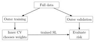
Nested cross-validation evaluates the entire Super Learner procedure.

If the same folds used to choose weights were also used to evaluate the final Super Learner, the risk estimate would be optimistic. Nested cross-validation avoids this by holding out outer validation observations from every part of fitting and weight selection.

46.3 Cross-Validated Risk Estimates

CV.SuperLearner() returns risk estimates for:

each candidate algorithm;
the discrete Super Learner;
the ensemble Super Learner.

For continuous outcomes with squared-error loss, the risk is estimated mean squared prediction error: \[\widehat R_{CV} = \frac{1}{n}\sum_{i=1}^n \{Y_i-\hat Q_{-v(i)}(A_i,W_i)\}^2,\] where \(\hat Q_{-v(i)}\) denotes the prediction rule trained without the outer validation fold containing observation \(i\).

46.4 Confidence Intervals for Risk

Plots from CV.SuperLearner() often display estimated risk and approximate confidence intervals. These intervals quantify uncertainty in the estimated predictive risk, not uncertainty in a causal effect. They are useful for judging whether apparent risk differences are meaningful or mostly noise.

If two algorithms have very similar risk estimates with overlapping intervals, it is not reasonable to claim that one is clearly better. The ensemble can still use both, or put weight on only one, depending on the metalearner optimization.

46.5 Discrete Super Learner

The discrete Super Learner is the single candidate with the best cross-validated risk. When evaluating results, it is helpful to compare: \[\text{best single candidate},\qquad \text{discrete Super Learner},\qquad \text{ensemble Super Learner}.\] In some datasets, the ensemble improves on all individual candidates. In others, the best single candidate performs about as well as the ensemble.

46.6 Comparing Super Learner to Candidate Algorithms

The following questions guide interpretation:

Does the ensemble have lower estimated risk than the best single candidate?
Are risk differences large relative to their uncertainty?
Which algorithms receive nonzero weight?
Are any algorithms unstable, slow, or producing warnings?
Does the selected library behave differently for \(\overline{Q}\) than for \(g\)?

Key Idea

SuperLearner() fits an ensemble for use in analysis. CV.SuperLearner() evaluates how well the entire ensemble-building procedure predicts new data.

Estimation Notes

For causal effect estimation, nested evaluation is a diagnostic for nuisance-function prediction. It does not prove that the resulting causal estimator is unbiased, because causal validity still depends on identification assumptions and adequate positivity.

Lecture 6.8. Reporting a Super Learner Analysis

47.1 Number of Folds

A report should state the number of cross-validation folds used to train and evaluate the Super Learner. Common choices are \(V=5\) and \(V=10\). If nested cross-validation was used, report both the outer folds and the inner folds.

For example, one might write:

The Super Learner was trained using ten-fold cross-validation to choose ensemble weights. Predictive performance of the full Super Learner procedure was evaluated using nested ten-fold cross-validation.

47.2 Candidate Algorithms

The candidate library is part of the estimator and must be reported. Include the algorithm names, important tuning parameters, and whether any variable screening procedures were paired with each learner.

\[\begin{array}{lll} \toprule \text{Learner} & \text{Description} & \text{Screener}\\ \midrule \texttt{SL.glm} & \text{main-terms GLM} & \text{All variables}\\ \texttt{SL.mean} & \text{intercept-only model} & \text{All variables}\\ \texttt{SL.ranger} & \text{random forest} & \text{All variables}\\ \texttt{SL.glm} & \text{main-terms GLM} & \texttt{screen.corP}\\ \bottomrule \end{array}\]

Large libraries are often best placed in an appendix table.

47.3 Ensemble Construction

State whether the analysis used a discrete Super Learner or an ensemble Super Learner. For ensemble Super Learner, describe the metalearner. For continuous outcomes, a convex least-squares ensemble is common. For binary outcomes or propensity scores, a logistic-linear ensemble minimizing negative log-likelihood is often appropriate.

47.4 Loss Functions

The loss function determines what the Super Learner is optimizing. Reports should state the loss separately for each nuisance function:

outcome regression with continuous \(Y\): mean squared-error loss;
outcome regression with binary \(Y\): Bernoulli negative log-likelihood or another valid binary-outcome loss;
propensity score: Bernoulli negative log-likelihood for treatment prediction.

47.5 Cross-Validated Risk Summaries

Risk summaries should include the Super Learner, the discrete Super Learner, and the candidate algorithms. A clear table includes the risk estimate, an uncertainty summary when available, and the ensemble weight.

\[\begin{array}{lccc} \toprule \text{Learner} & \text{CV risk} & \text{Weight} & \text{Comment}\\ \midrule \texttt{SL.glm\_All} & 1.03 & 0.40 & \text{stable benchmark}\\ \texttt{SL.mean\_All} & 2.72 & 0.00 & \text{intercept only}\\ \texttt{SL.quadglm\_All} & 1.05 & 0.60 & \text{quadratic terms}\\ \text{Super Learner} & 1.01 & -- & \text{ensemble}\\ \bottomrule \end{array}\]

47.6 Sensitivity Analyses

Super Learner results depend on the candidate library, loss function, and cross-validation design. Sensitivity analyses can examine whether conclusions change when:

additional flexible learners are added;
unstable or extremely slow learners are removed;
the number of folds is changed;
required confounders are forced into every candidate;
alternative reasonable losses are used;
propensity score learners producing extreme weights are excluded or modified.

47.7 Methods Write-Up

A concise methods paragraph for an outcome regression might read:

The outcome regression was estimated using Super Learner. Candidate algorithms included generalized linear models, penalized regression, generalized additive models, random forests, and multivariate adaptive regression splines, with selected learners paired with pre-specified screening rules. Ensemble weights were chosen to minimize ten-fold cross-validated mean squared-error loss using a convex least-squares metalearner.

For a propensity score:

The propensity score was estimated using Super Learner with treatment as the outcome and baseline covariates as predictors. Ensemble weights were chosen to minimize ten-fold cross-validated Bernoulli negative log-likelihood using a logistic-linear metalearner.

47.8 Results Write-Up

A results paragraph should summarize which learners contributed meaningfully and how the ensemble compared with individual candidates:

For the outcome regression, the Super Learner placed nonzero weight on five candidate algorithms, with the largest weights assigned to a random forest and a generalized additive model. Nested cross-validation suggested that the ensemble had lower estimated risk than any single candidate. For the propensity score, the ensemble performed similarly to the best individual learner, and predicted treatment probabilities showed no severe near-zero or near-one instability.

Avoid interpreting weights as evidence that a scientific model is true. They describe predictive contributions under the chosen loss.

47.9 Appendix Tables

Appendix tables should make the analysis reproducible. At minimum, include:

wrapper function names;
plain-language descriptions of each algorithm;
tuning parameters;
screening rules;
cross-validated risks;
Super Learner weights;
software versions when important.

Causal Assumption

Reporting Super Learner details does not replace reporting causal identification assumptions. The final causal analysis should separately state the target causal parameter, consistency, exchangeability, positivity, the adjustment set, and the statistical estimator.

Estimation Notes

A complete Super Learner report lets another analyst reconstruct the nuisance estimation procedure: folds, library, screeners, losses, metalearner, risk summaries, weights, and sensitivity analyses.

Chapter 7. Efficient, Doubly Robust Estimation of the ATE

Lecture 7.1. Limitations of Naive G-Computation and IPTW

48.1 Dependence on Nuisance Regression Consistency

The point-treatment ATE is identified, under consistency, conditional exchangeability, and positivity, by \[\operatorname{ATE}=\mathbb{E}\{\overline{Q}(1,W)-\overline{Q}(0,W)\}, \qquad \overline{Q}(a,w)=\mathbb{E}(Y\,\vert\,A=a,W=w),\] and also by inverse probability weighting: \[\mathbb{E}\{Y(a)\} = \mathbb{E}\left\{\frac{\mathbb{1}(A=a)}{g_a(W)}Y\right\}, \qquad g_a(w)=\mathbb{P}(A=a\,\vert\,W=w).\] These formulas lead directly to the estimators studied in Chapter 4: \[\psi_{n,G}(a)=\frac{1}{n}\sum_{i=1}^n\overline{Q}_n(a,W_i)\] and \[\psi_{n,\operatorname{IPTW}}(a)= \frac{1}{n}\sum_{i=1}^n \frac{\mathbb{1}(A_i=a)}{g_{n,a}(W_i)}Y_i.\]

Each estimator relies on consistent estimation of a nuisance regression. The g-computation estimator relies on \(\overline{Q}_n\) being close to \(\overline{Q}\). The IPTW estimator relies on \(g_{n,a}\) being close to \(g_a\). If the required nuisance function is estimated poorly, the resulting causal effect estimator can be biased even in large samples.

Causal Assumption

All estimators in this chapter require the same causal identification assumptions as before: \[Y=Y(A),\qquad Y(a)\perp\!\!\!\perp A\,\vert\,W,\qquad 0<\mathbb{P}(A=a\,\vert\,W=w)<1.\] Doubly robust estimation improves statistical robustness to nuisance-model misspecification; it does not remove the need for these causal assumptions.

48.2 Outcome Regression Misspecification

Suppose the analyst fits a main-terms outcome regression \[\overline{Q}_n(a,w)\approx \beta_0+\beta_1a+\beta_2w,\] but the true conditional mean contains an interaction: \[\overline{Q}(a,w)=\beta_0+\beta_1a+\beta_2w+\beta_3aw.\] Then \(\overline{Q}_n(1,w)-\overline{Q}_n(0,w)\) may be systematically wrong for some values of \(w\). Since g-computation averages these predicted contrasts over the covariate distribution, the resulting ATE estimator can converge to the wrong target.

This is not a small-sample problem. With enough data, the fitted main-terms model may converge very precisely to the best linear approximation within the misspecified model class. Precision around the wrong function is still bias for the causal estimand.

48.3 Propensity Score Misspecification

IPTW has a parallel vulnerability. If the propensity score model is misspecified, the weights \[\frac{\mathbb{1}(A_i=a)}{g_{n,a}(W_i)}\] do not create the intended pseudo-population. Some covariate strata may remain overrepresented and others underrepresented after weighting. In extreme cases, an incorrect propensity model can also create highly variable weights without correcting confounding.

For example, if the true propensity score is nonlinear, \[g_1(w)=\mathop{\mathrm{expit}}(\alpha_0+\alpha_1w+\alpha_2w^2),\] but the analyst fits \(\mathop{\mathrm{expit}}(\gamma_0+\gamma_1w)\), the fitted probabilities can be wrong exactly in regions where treatment assignment is most imbalanced.

48.4 Flexible Regression Complications

Super Learning and other flexible regression methods help reduce the risk of severe misspecification. They allow \(\overline{Q}_n\) and \(g_n\) to adapt to nonlinearities, interactions, and high-dimensional predictor structures.

However, flexible regression creates two new issues. First, flexible learners may converge more slowly than parametric estimators. Second, their sampling distributions can be difficult to characterize. The final causal estimator is no longer a simple average of independent terms with fixed nuisance functions; it contains data-adaptive estimated functions.

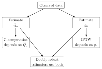
Naive g-computation and IPTW each depend on one nuisance function; doubly robust estimators combine both.

48.5 Lack of Standard Inference Basis

For a simple sample mean, the central limit theorem gives a standard basis for confidence intervals. For a parametric regression coefficient, classical regression theory gives approximate standard errors under model assumptions. For naive g-computation or IPTW with highly adaptive nuisance estimates, neither argument directly applies without additional work.

The statistical question is not only whether \(\psi_n\) is consistent. We also need an approximation of the form \[\sqrt n(\psi_n-\psi)\overset{d}{\longrightarrow}N(0,\sigma^2),\] and a consistent estimator of \(\sigma^2\). Doubly robust estimators are designed to have an asymptotic linear representation under appropriate conditions, which gives a direct route to inference.

48.6 Bootstrap Limitations

The nonparametric bootstrap is often useful, but it is not a universal remedy. With highly adaptive learners, variable selection, non-smooth tuning, or near-positivity violations, bootstrap distributions can fail to approximate the true sampling distribution. The bootstrap may also be computationally expensive because every bootstrap replicate must refit all nuisance functions.

Key Idea

The limitation of naive g-computation and IPTW is not that they are wrong as identification formulas. The limitation is that, as estimators, they rely heavily on one nuisance regression and do not automatically provide stable, valid inference when that nuisance regression is learned flexibly.

Lecture 7.2. Augmented IPTW Estimation

49.1 Combining G-Computation and IPTW

G-computation and IPTW use different nuisance functions. G-computation predicts counterfactual outcomes using \(\overline{Q}_n(a,w)\). IPTW reweights observed outcomes using \(g_{n,a}(w)\). Augmented inverse probability weighting combines both ideas in a single estimator.

The target counterfactual mean is \[\psi(a)=\mathbb{E}\{Y(a)\}.\] Under the usual identification assumptions, \[\psi(a)=\mathbb{E}\{\overline{Q}(a,W)\} = \mathbb{E}\left\{\frac{\mathbb{1}(A=a)}{g_a(W)}Y\right\}.\] The AIPTW estimator adds a residual correction to the g-computation estimator, or equivalently adds an outcome-regression correction to the IPTW estimator.

49.2 AIPTW Estimator for \(\mathbb{E}\{Y(1)\}\)

For treatment level \(1\), the AIPTW estimator is \[\psi_{n,\operatorname{AIPTW}}(1) = \frac{1}{n}\sum_{i=1}^n \left[ \overline{Q}_n(1,W_i) + \frac{\mathbb{1}(A_i=1)}{g_{n,1}(W_i)} \{Y_i-\overline{Q}_n(1,W_i)\} \right].\] The estimated ATE is obtained by forming the analogous estimator for treatment level \(0\) and subtracting: \[\widehat{\operatorname{ATE}}_{\operatorname{AIPTW}} = \psi_{n,\operatorname{AIPTW}}(1)-\psi_{n,\operatorname{AIPTW}}(0).\]

Estimation Notes

For binary treatment, \[\psi_{n,\operatorname{AIPTW}}(0) = \frac{1}{n}\sum_{i=1}^n \left[ \overline{Q}_n(0,W_i) + \frac{\mathbb{1}(A_i=0)}{g_{n,0}(W_i)} \{Y_i-\overline{Q}_n(0,W_i)\} \right],\] where \(g_{n,0}(W_i)=1-g_{n,1}(W_i)\).

49.3 IPTW Term

The estimator can be rearranged as \[\psi_{n,\operatorname{AIPTW}}(1) = \frac{1}{n}\sum_{i=1}^n \frac{\mathbb{1}(A_i=1)}{g_{n,1}(W_i)}Y_i + \frac{1}{n}\sum_{i=1}^n \left\{ 1-\frac{\mathbb{1}(A_i=1)}{g_{n,1}(W_i)} \right\} \overline{Q}_n(1,W_i).\] The first term is the usual IPTW estimator of \(\mathbb{E}\{Y(1)\}\): \[\frac{1}{n}\sum_{i=1}^n \frac{\mathbb{1}(A_i=1)}{g_{n,1}(W_i)}Y_i.\] It uses only observed treated outcomes, weighted by inverse treatment probabilities.

49.4 Augmentation Term

The second term, \[\frac{1}{n}\sum_{i=1}^n \left\{ 1-\frac{\mathbb{1}(A_i=1)}{g_{n,1}(W_i)} \right\} \overline{Q}_n(1,W_i),\] is the augmentation term. It uses the outcome regression to correct the IPTW estimator. If the estimated propensity score underweights or overweights certain treated individuals, the augmentation term offsets part of the resulting distortion.

For example, suppose \(Y\) is nonnegative and \(g_{n,1}(W)\) tends to underestimate the true probability of treatment. Then treated individuals receive weights that are too large, and the IPTW part tends to overshoot. The factor \(1-\mathbb{1}(A=1)/g_{n,1}(W)\) tends to be negative for treated observations with inflated weights, so the augmentation term can pull the estimate downward.

49.5 AIPTW as Augmented G-Computation

The same estimator can be viewed as g-computation plus a weighted residual average: \[\psi_{n,\operatorname{AIPTW}}(1) = \underbrace{ \frac{1}{n}\sum_{i=1}^n \overline{Q}_n(1,W_i) }_{\text{g-computation}} + \underbrace{ \frac{1}{n}\sum_{i=1}^n \frac{\mathbb{1}(A_i=1)}{g_{n,1}(W_i)} \{Y_i-\overline{Q}_n(1,W_i)\} }_{\text{augmentation}}.\] The augmentation is an average of observed residuals among treated individuals, weighted to represent the target population. If the outcome regression \(\overline{Q}_n(1,W)\) systematically overpredicts treated outcomes, then the residuals \(Y-\overline{Q}_n(1,W)\) tend to be negative, and the augmentation term lowers the g-computation estimate.

49.6 Intuition for Bias Correction

AIPTW uses \(\overline{Q}_n\) to predict missing counterfactual outcomes and uses \(g_n\) to check those predictions against observed residuals in the treatment group that actually reveals the relevant potential outcome. This creates a bias-correction mechanism.

AIPTW augments predicted counterfactual means with weighted residual corrections.

Key Idea

AIPTW is both augmented IPTW and augmented g-computation. The two algebraic forms are identical, but they highlight different sources of protection: the propensity score helps correct outcome-regression errors, and the outcome regression helps correct propensity-score errors.

Lecture 7.3. Double Robustness

50.1 Large-Sample Limits of AIPTW

Double robustness is a large-sample property. Suppose \[\overline{Q}_n(a,w)\overset{p}{\longrightarrow}\overline{Q}^*(a,w), \qquad g_{n,a}(w)\overset{p}{\longrightarrow}g_a^*(w),\] where \(\overline{Q}^*\) and \(g_a^*\) may or may not equal the true nuisance functions \(\overline{Q}\) and \(g_a\). For treatment level \(1\), the AIPTW estimator is expected to converge to \[H(\overline{Q}^*,g_1^*) = \mathbb{E}\left[ \overline{Q}^*(1,W) + \frac{\mathbb{1}(A=1)}{g_1^*(W)} \{Y-\overline{Q}^*(1,W)\} \right].\] The question is when this limit equals the target \(\mathbb{E}\{Y(1)\}\).

50.2 Correct Outcome Regression

First suppose the outcome regression is consistently estimated, so that \[\overline{Q}^*(1,W)=\overline{Q}(1,W)=\mathbb{E}(Y\,\vert\,A=1,W).\] Then \[\begin{aligned} H(\overline{Q},g_1^*) &= \mathbb{E}\left[ \overline{Q}(1,W) + \frac{\mathbb{1}(A=1)}{g_1^*(W)} \{Y-\overline{Q}(1,W)\} \right]\\ &= \mathbb{E}\left[ \overline{Q}(1,W) + \mathbb{E}\left\{ \frac{\mathbb{1}(A=1)}{g_1^*(W)} \{Y-\overline{Q}(1,W)\} \,\vert\,W \right\} \right]. \end{aligned}\] The inner expectation is zero because \[\begin{aligned} \mathbb{E}\left[ \mathbb{1}(A=1)\{Y-\overline{Q}(1,W)\} \,\vert\,W \right] &= \mathbb{P}(A=1\,\vert\,W) \mathbb{E}\{Y-\overline{Q}(1,W)\,\vert\,A=1,W\}\\ &= g_1(W)\{ \overline{Q}(1,W)-\overline{Q}(1,W)\}\\ &=0. \end{aligned}\] Therefore, \[H(\overline{Q},g_1^*)=\mathbb{E}\{\overline{Q}(1,W)\}=\mathbb{E}\{Y(1)\}.\] The propensity score limit may be wrong, but the estimator is still consistent if the outcome regression is correct.

50.3 Correct Propensity Score

Now suppose the propensity score is consistently estimated, so \(g_1^*(W)=g_1(W)\), but \(\overline{Q}^*\) may be wrong. Then \[\begin{aligned} H(\overline{Q}^*,g_1) &= \mathbb{E}\left[ \overline{Q}^*(1,W) + \frac{\mathbb{1}(A=1)}{g_1(W)} \{Y-\overline{Q}^*(1,W)\} \right]\\ &= \mathbb{E}\left[ \overline{Q}^*(1,W) + \mathbb{E}\left\{ \frac{\mathbb{1}(A=1)}{g_1(W)} \{Y-\overline{Q}^*(1,W)\} \,\vert\,W \right\} \right]. \end{aligned}\] Compute the inner expectation: \[\begin{aligned} \mathbb{E}\left[ \frac{\mathbb{1}(A=1)}{g_1(W)} \{Y-\overline{Q}^*(1,W)\} \,\vert\,W \right] &= \frac{1}{g_1(W)} \mathbb{E}\left[ \mathbb{1}(A=1)\{Y-\overline{Q}^*(1,W)\} \,\vert\,W \right]\\ &= \frac{g_1(W)}{g_1(W)} \{\overline{Q}(1,W)-\overline{Q}^*(1,W)\}\\ &= \overline{Q}(1,W)-\overline{Q}^*(1,W). \end{aligned}\] Substituting back, \[H(\overline{Q}^*,g_1) = \mathbb{E}\left[ \overline{Q}^*(1,W)+\overline{Q}(1,W)-\overline{Q}^*(1,W) \right] = \mathbb{E}\{\overline{Q}(1,W)\} = \mathbb{E}\{Y(1)\}.\]

50.4 Two Chances to Be Consistent

Definition 50.1 (Double robustness). An estimator is doubly robust for a parameter if it is consistent when either of two nuisance components is consistently estimated, even if the other nuisance component is inconsistently estimated.

For AIPTW, the two nuisance components are \(\overline{Q}\) and \(g\). The estimator of \(\mathbb{E}\{Y(1)\}\) is consistent if either \(\overline{Q}_n(1,w)\) is consistent for \(\overline{Q}(1,w)\) or \(g_{n,1}(w)\) is consistent for \(g_1(w)\). The same reasoning applies to \(\mathbb{E}\{Y(0)\}\) and therefore to the ATE.

Identification Result

Under the causal identification assumptions, the AIPTW estimator targets \(\mathbb{E}\{Y(a)\}\). Its large-sample limit equals this target if either \(\overline{Q}_n(a,w)\) consistently estimates \(\overline{Q}(a,w)\) or \(g_{n,a}(w)\) consistently estimates \(g_a(w)\).

50.5 Concrete Misspecification Example

A simple data-generating system makes the double-robustness statement operational. Suppose \[W\sim \operatorname{Uniform}(-2,2), \qquad A\,\vert\,W=w\sim \operatorname{Bernoulli}\{g_0(w)\},\] where \[g_0(w)=\operatorname{expit}\left\{\frac{3}{2}(w+1)^2-3\right\},\] and suppose the conditional mean outcome is \[\overline{Q}_0(a,w)=\mathbb{E}(Y\,\vert\,A=a,W=w)=1+a-w-aw.\] The true outcome regression contains an interaction between treatment and the covariate because of the term \(-aw\). A main-terms-only outcome regression, such as \(\mathbb{E}(Y\,\vert\,A,W)=\beta_0+\beta_1A+\beta_2W\), is therefore misspecified. The true propensity score is nonlinear in \(W\) because it contains \((w+1)^2\). A logistic propensity score model with only a linear term in \(W\) is therefore misspecified.

This example creates four useful cases: \[\begin{array}{c|c|c|c} \text{Outcome model} & \text{Propensity model} & \text{G-computation} & \text{IPTW}\\ \hline \text{correct} & \text{correct} & \text{consistent} & \text{consistent}\\ \text{correct} & \text{wrong} & \text{consistent} & \text{biased in general}\\ \text{wrong} & \text{correct} & \text{biased in general} & \text{consistent}\\ \text{wrong} & \text{wrong} & \text{biased in general} & \text{biased in general} \end{array}\] The AIPTW estimator is consistent in the first three rows, but not generally in the fourth row, where both nuisance models are wrong. In the second row, the augmentation term uses the correct outcome regression and the residual correction has mean zero. In the third row, the residual correction is weighted by the correct propensity score and removes the bias left by the wrong outcome regression. The fourth row is the warning case: double robustness gives two chances to remove bias, not a guarantee when both chances fail.

50.6 Why Double Robustness Is Not a License for Bad Models

Double robustness is sometimes summarized as “two chances to get it right.” That phrase is useful, but it can be misleading. If both nuisance estimators are poor, the AIPTW estimator can be badly biased. If both are estimated by simplistic parametric models that miss important nonlinearities or interactions, there may be no real second chance.

Double robustness also does not protect against violations of causal assumptions. Unmeasured confounding, interference, ill-defined interventions, or severe positivity violations can invalidate the causal interpretation regardless of the statistical estimator.

50.7 Connection to Efficiency

The AIPTW estimator is closely related to the efficient influence function for the counterfactual mean. When both nuisance functions are consistently estimated at sufficient rates, AIPTW can achieve the nonparametric efficiency bound for the target parameter. This means that, in large samples and under regularity conditions, no regular asymptotically linear estimator can have smaller asymptotic variance in the nonparametric model.

Key Idea

Double robustness concerns consistency under one correct nuisance function. Efficiency concerns variance when both nuisance functions are sufficiently well estimated. The same augmentation structure is responsible for both properties.

Lecture 7.4. AIPTW Implementation in R

51.1 Fitting the Outcome Regression

To compute AIPTW, first estimate the outcome regression \[\overline{Q}(a,w)=\mathbb{E}(Y\,\vert\,A=a,W=w).\] For a binary outcome, logistic regression is a simple starting point:

Implementation Notes

# dat contains Y, A, and W variables
or_fit <- glm(Y ~ A + W, data = dat, family = binomial())

dat1 <- dat
dat1$A <- 1
Qbar_1W <- predict(or_fit, newdata = dat1, type = "response")

dat0 <- dat
dat0$A <- 0
Qbar_0W <- predict(or_fit, newdata = dat0, type = "response")

The objects Qbar_1W and Qbar_0W are estimates of \(\overline{Q}(1,W_i)\) and \(\overline{Q}(0,W_i)\) for every observed individual.

51.2 Fitting the Propensity Score

Next estimate the propensity score: \[g_1(w)=\mathbb{P}(A=1\,\vert\,W=w).\]

Implementation Notes

ps_fit <- glm(A ~ W, data = dat, family = binomial())

g_1W <- predict(ps_fit, newdata = dat, type = "response")
g_0W <- 1 - g_1W

In practice, both \(\overline{Q}_n\) and \(g_n\) can be estimated using Super Learner. The subsequent AIPTW calculations are the same once predicted values are available.

51.3 Computing AIPTW for \(\mathbb{E}\{Y(1)\}\)

For treatment level \(1\), \[\psi_{n,\operatorname{AIPTW}}(1) = \frac{1}{n}\sum_{i=1}^n \left[ \overline{Q}_n(1,W_i) + \frac{\mathbb{1}(A_i=1)}{g_{n,1}(W_i)} \{Y_i-\overline{Q}_n(1,W_i)\} \right].\] In R:

Implementation Notes

A <- dat$A
Y <- dat$Y

aiptw_ey1 <- mean(Qbar_1W + (A == 1) / g_1W * (Y - Qbar_1W))

This expression is often safer than writing separate means for the g-computation and augmentation terms because it keeps the individual contribution visible.

51.4 Computing AIPTW for \(\mathbb{E}\{Y(0)\}\)

For treatment level \(0\), \[\psi_{n,\operatorname{AIPTW}}(0) = \frac{1}{n}\sum_{i=1}^n \left[ \overline{Q}_n(0,W_i) + \frac{\mathbb{1}(A_i=0)}{g_{n,0}(W_i)} \{Y_i-\overline{Q}_n(0,W_i)\} \right].\] In R:

Implementation Notes

aiptw_ey0 <- mean(Qbar_0W + (A == 0) / g_0W * (Y - Qbar_0W))

51.5 Computing the ATE

The AIPTW ATE estimator is \[\widehat{\operatorname{ATE}}_{\operatorname{AIPTW}} = \psi_{n,\operatorname{AIPTW}}(1)-\psi_{n,\operatorname{AIPTW}}(0).\]

Implementation Notes

aiptw_ate <- aiptw_ey1 - aiptw_ey0

Equivalently, define individual ATE contributions \[D_{i,n} = \overline{Q}_n(1,W_i)-\overline{Q}_n(0,W_i) + \frac{A_i}{g_{n,1}(W_i)}\{Y_i-\overline{Q}_n(1,W_i)\} - \frac{1-A_i}{g_{n,0}(W_i)}\{Y_i-\overline{Q}_n(0,W_i)\}.\] Then \[\widehat{\operatorname{ATE}}_{\operatorname{AIPTW}}=\frac{1}{n}\sum_{i=1}^nD_{i,n}.\]

51.6 Practical Coding Workflow

Estimation Notes

AIPTW coding workflow:

Fit or otherwise estimate \(\overline{Q}_n(A,W)\).
Predict \(\overline{Q}_n(1,W_i)\) and \(\overline{Q}_n(0,W_i)\) for every individual.
Fit or otherwise estimate \(g_{n,1}(W)\).
Compute \(g_{n,0}(W_i)=1-g_{n,1}(W_i)\).
Form \(\psi_{n,\operatorname{AIPTW}}(1)\) and \(\psi_{n,\operatorname{AIPTW}}(0)\).
Subtract to estimate the ATE.
Compute influence-function-based standard errors as described in the next lecture.

Always check the range of estimated propensity scores. Extremely small values of \(g_{n,1}(W_i)\) among treated observations or \(g_{n,0}(W_i)\) among untreated observations can create unstable residual corrections.

Implementation Notes

summary(g_1W)
summary(g_0W)
summary((A == 1) / g_1W)
summary((A == 0) / g_0W)

Lecture 7.5. Influence-Function-Based Inference

52.1 Asymptotic Linearity

An estimator \(\psi_n\) is asymptotically linear for a parameter \(\psi\) if it can be written as \[\psi_n-\psi = \frac{1}{n}\sum_{i=1}^n D(O_i)+o_p(n^{-1/2}),\] where \(D(O)\) has mean zero and finite variance. The function \(D\) is an influence function. This representation implies \[\sqrt n(\psi_n-\psi)\overset{d}{\longrightarrow} N\{0,\mathop{\mathrm{Var}}(D(O))\}.\]

For the counterfactual mean \(\psi(1)=\mathbb{E}\{Y(1)\}\), the efficient influence function under the nonparametric point-treatment model is \[D_1(O) = \frac{\mathbb{1}(A=1)}{g_1(W)} \{Y-\overline{Q}(1,W)\} + \overline{Q}(1,W)-\psi(1).\] For \(\psi(0)\), \[D_0(O) = \frac{\mathbb{1}(A=0)}{g_0(W)} \{Y-\overline{Q}(0,W)\} + \overline{Q}(0,W)-\psi(0).\] For the ATE, the influence function is \[D_{\operatorname{ATE}}(O)=D_1(O)-D_0(O).\]

52.2 Estimated Influence Function

In practice, replace unknown quantities by estimates. For \(\psi(1)\): \[D_{1,n}(O_i) = \frac{\mathbb{1}(A_i=1)}{g_{n,1}(W_i)} \{Y_i-\overline{Q}_n(1,W_i)\} + \overline{Q}_n(1,W_i)-\psi_{n,\operatorname{AIPTW}}(1).\] For \(\psi(0)\): \[D_{0,n}(O_i) = \frac{\mathbb{1}(A_i=0)}{g_{n,0}(W_i)} \{Y_i-\overline{Q}_n(0,W_i)\} + \overline{Q}_n(0,W_i)-\psi_{n,\operatorname{AIPTW}}(0).\] For the ATE: \[D_{\operatorname{ATE},n}(O_i)=D_{1,n}(O_i)-D_{0,n}(O_i).\]

52.3 Variance Estimation

Estimate the asymptotic variance of \(\psi_n(1)\) by the empirical variance of the estimated influence function: \[\hat\tau_1^2 = \frac{1}{n}\sum_{i=1}^n D_{1,n}(O_i)^2.\] The standard error is \[\widehat{\mathrm{SE}}\{\psi_n(1)\} = \sqrt{\hat\tau_1^2/n}.\] For the ATE, use \[\hat\tau_{\operatorname{ATE}}^2 = \frac{1}{n}\sum_{i=1}^n \left\{ D_{\operatorname{ATE},n}(O_i)-\bar D_{\operatorname{ATE},n} \right\}^2,\] where \(\bar D_{\operatorname{ATE},n}=n^{-1}\sum_iD_{\operatorname{ATE},n}(O_i)\), and \[\widehat{\mathrm{SE}}(\widehat{\operatorname{ATE}}) = \sqrt{\hat\tau_{\operatorname{ATE}}^2/n}.\] For AIPTW, \(\bar D_{\operatorname{ATE},n}\) is usually very close to zero by construction, but centering is harmless and often used in software.

52.4 Wald Confidence Intervals

An approximate 95% Wald interval for \(\psi(1)\) is \[\psi_{n,\operatorname{AIPTW}}(1) \pm 1.96\sqrt{\hat\tau_1^2/n}.\] An approximate 95% interval for the ATE is \[\widehat{\operatorname{ATE}}_{\operatorname{AIPTW}} \pm 1.96\,\widehat{\mathrm{SE}}(\widehat{\operatorname{ATE}}).\]

Implementation Notes

Influence-function standard error for the ATE:

D1 <- (A == 1) / g_1W * (Y - Qbar_1W) + Qbar_1W - aiptw_ey1
D0 <- (A == 0) / g_0W * (Y - Qbar_0W) + Qbar_0W - aiptw_ey0
Date <- D1 - D0

se_ate <- sqrt(var(Date) / length(Y))
ci_ate <- aiptw_ate + c(-1.96, 1.96) * se_ate

52.5 Hypothesis Tests

For testing \[H_0:\operatorname{ATE}=0 \qquad\text{versus}\qquad H_1:\operatorname{ATE}\neq 0,\] use \[Z=\frac{\widehat{\operatorname{ATE}}_{\operatorname{AIPTW}}} {\widehat{\mathrm{SE}}(\widehat{\operatorname{ATE}})}.\] The two-sided Wald p-value is \[p=2\{1-\Phi(|Z|)\},\] where \(\Phi\) is the standard normal distribution function.

52.6 Coverage in Finite Samples

Influence-function inference is asymptotic. In finite samples, coverage can be below or above the nominal level if nuisance regressions are unstable, positivity is weak, or the sample size is too small for the normal approximation. Coverage often improves as \(n\) grows, provided the nuisance estimators and regularity conditions are adequate.

The estimated influence-function values should be inspected. A few extremely large values can indicate that confidence intervals are being driven by near-zero propensity scores or extreme residuals.

52.7 Simulation Interpretation

Simulation studies often compare the empirical coverage probability of nominal 95% confidence intervals. If 1000 simulated datasets are generated and the 95% interval contains the true parameter in 946 of them, the estimated coverage probability is 94.6%. Such studies reveal finite-sample behavior of the estimator and interval, not whether a single real-data analysis satisfies the causal assumptions.

Key Idea

The influence function turns a complicated doubly robust estimator into an approximate sample mean of mean-zero terms. This is the basis for standard errors, Wald intervals, and p-values.

Lecture 7.6. Use in Randomized Trials

53.1 Why Covariate Adjustment Can Improve Precision

In a randomized trial, treatment assignment is controlled by design. If treatment is randomized with probability \(p\), then \[A\perp\!\!\!\perp W,\qquad \mathbb{P}(A=1\,\vert\,W)=p.\] Because treatment is randomized, the unadjusted difference in means is consistent for the ATE: \[\hat\psi_{\mathrm{unadj}} = \frac{\sum_iY_i\mathbb{1}(A_i=1)}{\sum_i\mathbb{1}(A_i=1)} - \frac{\sum_iY_i\mathbb{1}(A_i=0)}{\sum_i\mathbb{1}(A_i=0)}.\]

Covariate adjustment is not required to remove confounding in a well-conducted randomized trial. It can still improve precision. If baseline covariates strongly predict the outcome, adjusting for them can remove outcome variation unrelated to treatment, leading to smaller standard errors.

53.2 Known Propensity Score Under Randomization

In a trial with known randomization probability \(p\), \[g_1(W)=p,\qquad g_0(W)=1-p.\] For equal randomization, \(p=0.5\). In AIPTW, the known propensity score can be used instead of estimating \(g\): \[\psi_{n,\operatorname{AIPTW}}(1) = \frac{1}{n}\sum_{i=1}^n \left[ \overline{Q}_n(1,W_i) + \frac{A_i}{p}\{Y_i-\overline{Q}_n(1,W_i)\} \right].\] The corresponding expression for \(a=0\) uses \((1-A_i)/(1-p)\).

Causal Assumption

In a randomized trial, exchangeability follows from the randomization design only for the trial population and intervention actually randomized. Other issues, such as nonadherence, loss to follow-up, interference, or changes in the target population, require additional causal assumptions.

53.3 Efficiency Gains

If \(\overline{Q}_n\) predicts \(Y\) well, the residuals \(Y-\overline{Q}_n(A,W)\) are less variable than the raw outcomes. AIPTW and TMLE use this predictive information while preserving validness through the known randomization probability. The gain is largest when baseline covariates are strongly prognostic.

For equal randomization and a well-estimated outcome regression, the precision gain depends on how much variation in the outcome is explained by baseline covariates and how treatment effects vary with covariates.

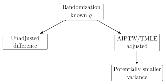
In randomized trials, adjustment is used for precision rather than confounding control.

53.4 Outcome Regression in Randomized Trials

The outcome regression in a trial can include baseline covariates and treatment: \[\overline{Q}(a,w)=\mathbb{E}(Y\,\vert\,A=a,W=w).\] It may include treatment-covariate interactions if effect heterogeneity is plausible. Because the propensity score is known, double robustness implies that consistency of AIPTW does not require the outcome regression to be correct. However, a poor outcome regression can fail to improve precision and may slightly harm finite-sample performance.

53.5 When Doubly Robust Methods Are Useful Even Without Confounding

Doubly robust methods are useful in randomized trials because they provide:

design-protected consistency through the known \(g\);
valid influence-function inference under mild conditions;
possible efficiency gains from prognostic baseline covariates;
a unified analysis strategy that extends naturally to trials with unequal randomization or covariate-adaptive designs.

Key Idea

In observational studies, adjustment is needed for identification. In randomized trials, adjustment is often used for efficiency. The same AIPTW and TMLE formulas apply, but the known randomization probability gives a particularly strong foundation.

Lecture 7.7. Targeted Minimum Loss-Based Estimation

54.1 Compatible Plug-In Estimators

A compatible plug-in estimator is an estimator that can be written as a parameter mapping applied to an estimated distribution. For example, the g-computation estimator \[\psi_{n,G}(1)=\frac{1}{n}\sum_{i=1}^n\overline{Q}_n(1,W_i)\] is a plug-in estimator: it applies the counterfactual mean mapping to an estimated outcome regression and empirical covariate distribution.

IPTW and AIPTW are not generally plug-in estimators in this sense. They can produce values outside natural parameter bounds. For example, for a binary outcome, a counterfactual mean should lie in \([0,1]\), but a weighted residual estimator can in finite samples fall outside that interval.

54.2 Motivation for TMLE

Targeted minimum loss-based estimation constructs a plug-in estimator with influence-function-based bias correction. The idea is to start with an initial outcome regression \(\overline{Q}_n\), then update it in a targeted way so that the empirical mean of the efficient influence function is approximately zero.

For \(\psi(1)\), the relevant residual equation is \[0= \frac{1}{n}\sum_{i=1}^n \frac{\mathbb{1}(A_i=1)}{g_{n,1}(W_i)} \{Y_i-\overline{Q}_n^*(1,W_i)\}.\] If the updated regression \(\overline{Q}_n^*\) satisfies this equation and remains a valid conditional mean, then the plug-in estimator \[\psi_{n,\operatorname{TMLE}}(1)=\frac{1}{n}\sum_{i=1}^n\overline{Q}_n^*(1,W_i)\] inherits the same first-order bias correction as AIPTW while preserving parameter constraints.

54.3 Initial Outcome Regression

TMLE begins by estimating \(\overline{Q}(A,W)\) and \(g_1(W)\). These can be estimated using parametric models or flexible learners such as Super Learner. For a bounded or binary outcome, the initial outcome regression should produce predictions inside \((0,1)\).

54.4 Targeting Step

For simplicity, consider a binary outcome and estimation of \(\psi(1)\). Let \[K_i=\mathop{\mathrm{logit}}\{\overline{Q}_n(1,W_i)\}\] be the offset and define the clever covariate \[H_1(A_i,W_i)=\frac{\mathbb{1}(A_i=1)}{g_{n,1}(W_i)}.\] Fit a logistic regression with outcome \(Y\), offset \(K_i\), and single covariate \(H_1(A_i,W_i)\), often using only observations with \(A_i=1\) for this one-treatment update. The fitted coefficient is denoted \(\hat\epsilon\). Logistic fluctuation is directly natural for binary outcomes or outcomes scaled to \([0,1]\); for continuous unbounded outcomes, TMLE should use an appropriate loss and submodel or transform the outcome before using a bounded-loss formulation.

54.5 Clever Covariate

The clever covariate is called “clever” because it is chosen from the efficient influence function. For treatment level \(1\), \[H_1(A,W)=\frac{\mathbb{1}(A=1)}{g_1(W)}.\] It weights the outcome-regression fluctuation so that the updated regression solves the empirical residual equation associated with \(\psi(1)\).

54.6 Updated Regression

The updated regression for treatment level \(1\) is \[\overline{Q}_n^*(1,w) = \mathop{\mathrm{expit}}\left[ \mathop{\mathrm{logit}}\{\overline{Q}_n(1,w)\} + \hat\epsilon\frac{1}{g_{n,1}(w)} \right].\] More generally, to target both \(\psi(1)\) and \(\psi(0)\) simultaneously, define \[H_1(A,W)=\frac{A}{g_{n,1}(W)},\qquad H_0(A,W)=\frac{1-A}{g_{n,0}(W)}.\] Fit a logistic fluctuation model with offset \(\mathop{\mathrm{logit}}\{\overline{Q}_n(A,W)\}\) and covariates \(H_1\) and \(H_0\). If the fitted coefficients are \(\hat\epsilon_1\) and \(\hat\epsilon_0\), then \[\overline{Q}_n^*(a,w) = \mathop{\mathrm{expit}}\left[ \mathop{\mathrm{logit}}\{\overline{Q}_n(a,w)\} + \hat\epsilon_1\frac{a}{g_{n,1}(w)} + \hat\epsilon_0\frac{1-a}{g_{n,0}(w)} \right].\]

54.7 TMLE Estimate

The TMLE counterfactual means are plug-in estimates: \[\psi_{n,\operatorname{TMLE}}(1) = \frac{1}{n}\sum_{i=1}^n\overline{Q}_n^*(1,W_i),\] \[\psi_{n,\operatorname{TMLE}}(0) = \frac{1}{n}\sum_{i=1}^n\overline{Q}_n^*(0,W_i),\] and \[\widehat{\operatorname{ATE}}_{\operatorname{TMLE}} = \psi_{n,\operatorname{TMLE}}(1)-\psi_{n,\operatorname{TMLE}}(0).\]

Implementation Notes

Conceptual TMLE code for a binary outcome:

H1 <- A / g_1W
H0 <- (1 - A) / g_0W
K  <- qlogis(Qbar_AW)

target_fit <- glm(Y ~ -1 + offset(K) + H1 + H0,
                  family = binomial(),
                  start = c(0, 0))

eps1 <- coef(target_fit)["H1"]
eps0 <- coef(target_fit)["H0"]

Qstar_1W <- plogis(qlogis(Qbar_1W) + eps1 / g_1W)
Qstar_0W <- plogis(qlogis(Qbar_0W) + eps0 / g_0W)

tmle_ate <- mean(Qstar_1W - Qstar_0W)

54.8 TMLE vs AIPTW

AIPTW and TMLE have the same efficient influence function under standard conditions. Both are doubly robust for consistency. The key difference is that TMLE is a targeted plug-in estimator. For bounded outcomes, it respects the natural bounds of the parameter. It can also have better finite-sample behavior in settings with practical positivity concerns.

Key Idea

TMLE updates the initial outcome regression just enough to solve the efficient influence-function estimating equation, then estimates the causal parameter by plugging in the updated regression.

Lecture 7.8. Doubly Robust Inference with Flexible Learners

55.1 Flexible Nuisance Estimation

Flexible learners are attractive because they reduce reliance on simple parametric models for \(\overline{Q}\) and \(g\). However, flexible nuisance estimation complicates inference. Consistency of AIPTW or TMLE can hold if either nuisance function is consistently estimated, but standard Wald inference usually requires more: a tractable asymptotic linear expansion with consistently estimable variance.

When both nuisance functions are consistently estimated at adequate rates, standard AIPTW and standard TMLE often have valid influence-function-based inference. The harder question is what happens when only one nuisance function is consistently estimated and flexible methods are used.

55.2 Standard TMLE

Standard TMLE targets the efficient influence function equation \[\frac{1}{n}\sum_{i=1}^nD_n^*(O_i)\approx 0,\] where \(D_n^*\) is the efficient influence function with \(\overline{Q}_n^*\) and \(g_n\) plugged in. This targeting step gives TMLE the same first-order expansion as AIPTW when the nuisance estimators behave well.

Standard TMLE is doubly robust for consistency: if either \(\overline{Q}_n\) or \(g_n\) is consistent, the parameter estimate can still be consistent. But this does not automatically guarantee valid confidence intervals when the other nuisance estimator is inconsistent and flexible estimation is used.

55.3 TMLE for Doubly Robust Inference

Doubly robust inference means more than doubly robust consistency. It means the estimator has a usable asymptotic normal distribution and variance estimator even when only one nuisance component is consistently estimated.

Specialized TMLEs can be constructed to target additional equations beyond the usual efficient influence-function equation. These methods may update both the outcome regression and the propensity score, often iteratively, to remove additional second-order terms that would otherwise prevent valid inference.

The technical details are advanced, but the practical message is clear: standard AIPTW and standard TMLE should not be assumed to deliver valid inference under arbitrary flexible nuisance estimation if one nuisance function is badly inconsistent.

55.4 Sample-Size Effects

Finite-sample performance depends strongly on sample size. In small samples, flexible learners can overfit, estimated propensity scores can be unstable, and influence-function approximations can be poor. As sample size grows, flexible regression can better approximate the nuisance functions, and coverage of influence-function intervals often improves.

The rate at which coverage improves depends on the complexity of the true nuisance functions, the learner library, positivity, and the amount of outcome noise.

55.5 Coverage Probability

Coverage probability is the repeated-sampling probability that a confidence interval contains the true parameter. A nominal 95% interval has good coverage if, across many repeated samples, it contains the target about 95% of the time.

Simulation studies comparing naive g-computation, standard TMLE, and TMLE designed for doubly robust inference often show that coverage can be poor at small sample sizes, especially when one nuisance regression is misspecified. Methods designed for doubly robust inference can improve coverage in such settings, but they are more complex and require careful implementation.

55.6 Practical Cautions

Estimation Notes

Practical guidance for flexible doubly robust estimation:

Use rich but pre-specified nuisance-function libraries.
Inspect estimated propensity scores and clever covariates for extreme values.
Use cross-fitting or sample splitting when required by the estimator’s theory.
Report whether inference relies on both nuisance functions being consistently estimated or on a method designed for doubly robust inference.
Treat small-sample Wald intervals cautiously when weights or influence-function values are highly variable.

Flexible learners are valuable, but they do not make inference automatic. The more adaptive the nuisance estimation procedure, the more important it is to use an estimator and inference procedure whose theoretical conditions match the analysis.

Key Idea

Doubly robust consistency says that the point estimator can remain consistent if one nuisance function is correct. Doubly robust inference is stronger: it asks for valid standard errors and confidence intervals under that same one-correct-nuisance scenario.

Causal Assumption

No amount of flexible nuisance estimation can diagnose unmeasured confounding from the observed data alone. Doubly robust inference concerns statistical robustness after identification assumptions have been accepted.

Chapter 8. Identification and Inference for Time-Varying Interventions

Lecture 8.1. Longitudinal Causal Questions

56.1 Multi-Timepoint Treatments

Many important interventions are not single decisions. A patient may take a medication every day, receive chemotherapy at several cycles, return for repeated injections, or decide whether to continue a behavioral program at each visit. In such settings the causal question concerns a sequence of treatment decisions, not only one baseline exposure.

Let time be indexed by \(k=0,1,\ldots,K\). At time \(k\), an individual has a recorded history, receives or does not receive treatment, and then continues to the next time point. The final outcome \(Y\) is observed after the last treatment decision.

A generic longitudinal treatment process. Covariates and treatments alternate over time before the final outcome.

Key Idea

A longitudinal causal question asks what would happen if the entire treatment history were set by an intervention. The unit of intervention is the treatment regime \(\overline{a}=(a_0,\ldots,a_K)\), not a single treatment indicator.

56.2 Longitudinal Data Structure

For one individual, write the observed data as \[O=(L_0,A_0,L_1,A_1,\ldots,L_K,A_K,Y).\] For \(n\) independent individuals, the sample is \[O_1,\ldots,O_n \overset{\mathrm{iid}}{\sim}P_0,\] where \(P_0\) denotes the true observed-data distribution. The variables have the following roles: \[L_k = \text{covariates recorded at time } k,\qquad A_k = \text{treatment at time } k,\qquad Y = \text{final outcome}.\] The covariate \(L_k\) may include new measurements, updated disease severity, adverse events, adherence information, symptoms, laboratory values, and summaries of earlier history. It is often vector-valued.

Notation 85. We use overbars for histories: \[\overline{L}_k=(L_0,\ldots,L_k),\qquad \overline{A}_k=(A_0,\ldots,A_k).\] For fixed treatment values, \[\overline{l}_k=(l_0,\ldots,l_k),\qquad \overline{a}_k=(a_0,\ldots,a_k).\] When the full treatment history is meant, \(\overline{A}=\overline{A}_K\) and \(\overline{a}=\overline{a}_K\).

The timing convention matters. In these notes, \(L_k\) is measured before \(A_k\). Thus \(A_k\) may depend on \(\overline{L}_k\) and \(\overline{A}_{k-1}\), but not on future covariates or future outcomes. This convention is not merely bookkeeping: it determines what information can be used by a treatment rule at time \(k\).

56.3 \(L_k\), \(A_k\), and \(Y\)

The variable \(L_k\) can be both a confounder and an intermediate. For example, baseline treatment \(A_0\) may affect a later biomarker \(L_1\), and that biomarker may affect both later treatment \(A_1\) and the outcome \(Y\). This feedback is a central reason why longitudinal causal inference requires special methods.

For two treatment times, the observed data are \[O=(L_0,A_0,L_1,A_1,Y).\] A typical causal ordering is \[L_0 \rightarrow A_0 \rightarrow L_1 \rightarrow A_1 \rightarrow Y,\] with additional arrows from earlier variables to later variables. The later covariate \(L_1\) is post-treatment with respect to \(A_0\), but pre-treatment with respect to \(A_1\).

56.4 Treatment Regimes

Definition 56.2 (Static treatment regime). A static treatment regime is a fixed vector \[\overline{a}=(a_0,\ldots,a_K)\] that assigns the same treatment value at each time point to every individual, regardless of the individual’s evolving covariate history.

Examples include “always treat,” represented by \((1,1,\ldots,1)\), and “never treat,” represented by \((0,0,\ldots,0)\) for a binary treatment. Other static regimes are possible, such as treating only during the first two visits and then stopping.

Definition 56.3 (Dynamic treatment regime). A dynamic treatment regime is a sequence of decision rules \[d=(d_0,\ldots,d_K),\] where \(d_k\) maps the information available at time \(k\) to a treatment value: \[A_k=d_k(\overline{L}_k,\overline{A}_{k-1}).\]

Dynamic regimes are discussed in detail in Section 66. For now, the key point is that longitudinal notation can handle both fixed treatment profiles and rules that respond to patient history.

56.5 Counterfactual Outcomes \(Y(a_0,\ldots,a_K)\)

Definition 56.4 (Longitudinal counterfactual outcome). For a fixed treatment regime \(\overline{a}=(a_0,\ldots,a_K)\), the counterfactual outcome \(Y(\overline{a})\) is the outcome that would be observed for an individual if, possibly contrary to fact, treatment were set to \(a_k\) at every time \(k=0,\ldots,K\).

For example, \(Y(1,1)\) is the outcome that would be observed under treatment at both time 0 and time 1. If the observed data contain \(A_0=1\) and \(A_1=0\), then \(Y(1,1)\) is not directly observed for that individual, even though \(Y(1,0)\) may be linked to the observed outcome by consistency.

Common population-level causal parameters include \[\psi(\overline{a})=\mathbb{E}\{Y(\overline{a})\},\] and contrasts such as \[\mathbb{E}\{Y(1,\ldots,1)\}-\mathbb{E}\{Y(0,\ldots,0)\}.\] For a binary outcome, this contrast is a risk difference comparing two entire treatment strategies.

56.6 Clinical Examples

Example 56.5 (Weekly osteoporosis therapy). Suppose \(A_k\) indicates whether a patient took alendronate during week \(k\), where \(k=0,\ldots,52\). Let \(L_k\) include age, prior fracture status, recent bone density measurements, thyroid hormone use, side effects, and other clinical information available at week \(k\). Let \(Y\) indicate whether hip fracture occurs within one year. A static contrast of interest is \[\mathbb{E}\{Y(1,1,\ldots,1)\}-\mathbb{E}\{Y(0,0,\ldots,0)\},\] the difference in one-year fracture risk under weekly therapy for the whole year versus no therapy during the year.

Example 56.6 (Cancer treatment continuation). At each chemotherapy cycle, \(A_k\) may indicate whether treatment is continued. The covariate \(L_k\) may include tumor response, toxicity, blood counts, and functional status. Treatment discontinuation may be caused by lack of response, and lack of response also predicts mortality. Thus later treatment decisions are confounded by earlier treatment-induced covariates.

Example 56.7 (Smoking cessation). Let \(A_k\) indicate whether an individual smokes during month \(k\). Respiratory symptoms recorded in \(L_k\) may lead a person to quit smoking and may also be early signs of disease. A comparison of sustained smoking versus sustained cessation must handle the fact that symptoms are both affected by prior smoking and predictive of later smoking and future outcomes.

Lecture 8.2. Sequential Identification Assumptions

57.1 Sequential Randomized Trials

The cleanest way to learn the mean counterfactual outcome \(\mathbb{E}\{Y(\overline{a})\}\) is to run a trial that randomizes treatment at each time point. In a sequentially randomized trial, treatment \(A_k\) is assigned by a known randomization mechanism after observing the history available at time \(k\).

For a fixed regime \(\overline{a}=(a_0,\ldots,a_K)\), randomization implies that treatment at each time is independent of the relevant counterfactual outcome within the history strata used by the trial: \[Y(\overline{a}) \perp\!\!\!\perp A_k \,\vert\,\overline{L}_k,\overline{A}_{k-1} \qquad \text{for } k=0,\ldots,K.\] At \(k=0\), the conditioning set is just \(L_0\).

Plainly, among people with the same history up to time \(k\), the next treatment assignment is as if randomized with respect to what would happen under the regime \(\overline{a}\). This is the longitudinal analogue of conditional randomization for a point treatment.

57.2 Observational Longitudinal Studies

In observational longitudinal studies, treatment is not assigned by the analyst. Patients and clinicians make decisions using information that evolves over time. Some of this information is measured and included in \(\overline{L}_k\); some may be unmeasured.

The inferential challenge is that the observed treatment process may be informative about future outcomes. For example, a patient may discontinue chemotherapy because disease is progressing, or a smoker may quit because early respiratory symptoms have appeared. If those health changes are also associated with the final outcome, treated and untreated histories are not automatically comparable.

57.3 Time-Varying Confounding

Definition 57.1 (Time-varying confounder). A time-varying confounder is a covariate \(L_k\) that predicts later treatment \(A_k\) or \(A_{k+1}\) and also predicts the outcome, while possibly being affected by earlier treatment.

This dual role is what makes longitudinal confounding different from ordinary baseline confounding. A later covariate can be necessary for controlling confounding of later treatment, yet inappropriate to condition on naively when estimating effects of earlier treatment because it lies on a causal pathway from earlier treatment to the outcome.

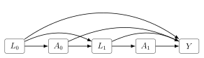
Treatment-confounder feedback: \(L_1\) is affected by \(A_0\) and also confounds the effect of \(A_1\) on \(Y\).

57.4 Sequential Randomization

Causal Assumption

For a fixed static regime \(\overline{a}=(a_0,\ldots,a_K)\), the sequential randomization assumption is \[Y(\overline{a}) \perp\!\!\!\perp A_k \,\vert\,\overline{L}_k,\overline{A}_{k-1}=\overline{a}_{k-1} \qquad k=0,\ldots,K.\] Equivalently, among individuals whose observed treatment history has followed the regime through time \(k-1\), the next treatment decision is independent of the counterfactual outcome under the full regime after conditioning on the measured covariate history.

The restriction \(\overline{A}_{k-1}=\overline{a}_{k-1}\) appears because, when identifying \(Y(\overline{a})\), the relevant risk set at time \(k\) consists of individuals who have remained compatible with the regime up to that time. If a person has already deviated from the regime, later treatment decisions for that person do not directly reveal outcomes under the full regime \(\overline{a}\) without further modeling.

57.5 Sequential Exchangeability

Sequential exchangeability is another name for the same identifying condition. It emphasizes comparability: after conditioning on the measured history, those who receive \(A_k=a_k\) and those who do not are exchangeable with respect to the future counterfactual outcome under \(\overline{a}\).

For two treatment times and regime \((1,1)\), the assumption is \[Y(1,1) \perp\!\!\!\perp A_0 \,\vert\,L_0,\] and \[Y(1,1) \perp\!\!\!\perp A_1 \,\vert\,L_0,A_0=1,L_1.\] The first line says baseline treatment is unconfounded within baseline covariate strata. The second says the second treatment is unconfounded within strata of the history observed among people treated at baseline.

This assumption is not empirically verifiable. The observed data can show whether treatment depends on measured covariates, but cannot show whether treatment depends on unmeasured determinants of the counterfactual outcome.

57.6 Longitudinal Positivity

Causal Assumption

For every history with positive probability under the regime of interest, the probability of receiving the regime-compatible treatment must be positive: \[\mathbb{P}(A_k=a_k \,\vert\,\overline{L}_k=\overline{l}_k,\overline{A}_{k-1}=\overline{a}_{k-1})>0 \qquad k=0,\ldots,K.\]

For the always-treated regime \((1,\ldots,1)\) this becomes \[\mathbb{P}(A_0=1\,\vert\,L_0=l_0)>0,\] \[\mathbb{P}(A_1=1\,\vert\,\overline{L}_1=\overline{l}_1,A_0=1)>0,\] and so on through time \(K\).

Longitudinal positivity is more fragile than single-timepoint positivity because probabilities multiply over time. Even if every time-specific probability is moderate, the probability of observing the entire treatment sequence can be small: \[\prod_{k=0}^K \mathbb{P}(A_k=a_k\,\vert\,\overline{L}_k,\overline{A}_{k-1}=\overline{a}_{k-1}).\] Small products lead to unstable inverse probability weights and can make some static regimes impossible to learn in a given population.

Key Idea

Identification of a longitudinal regime requires local exchangeability and local positivity at every treatment decision. A failure at one time point can break identification of the entire treatment sequence.

Lecture 8.3. Longitudinal G-Computation Formula

58.1 Two-Timepoint Derivation

Consider the observed data \[O=(L_0,A_0,L_1,A_1,Y)\] and the target parameter \[\psi(1,1)=\mathbb{E}\{Y(1,1)\}.\] Assume the three identifying conditions hold: consistency, sequential exchangeability, and positivity. The formula repeatedly replaces counterfactual conditional means with observed conditional means, then averages over the relevant covariate distributions.

Start with the innermost observed outcome regression: \[\mathbb{E}(Y\,\vert\,A_1=1,L_1,A_0=1,L_0).\] By consistency, among individuals with \(A_0=1\) and \(A_1=1\), the observed outcome equals \(Y(1,1)\). Therefore \[\mathbb{E}(Y\,\vert\,A_1=1,L_1,A_0=1,L_0) = \mathbb{E}\{Y(1,1)\,\vert\,A_1=1,L_1,A_0=1,L_0\}.\] By sequential exchangeability at time 1, \[Y(1,1)\perp\!\!\!\perp A_1\,\vert\,L_0,A_0=1,L_1,\] so \[\mathbb{E}\{Y(1,1)\,\vert\,A_1=1,L_1,A_0=1,L_0\} = \mathbb{E}\{Y(1,1)\,\vert\,L_1,A_0=1,L_0\}.\] Define \[\overline{Q}_2(L_0,L_1) = \mathbb{E}(Y\,\vert\,A_1=1,L_1,A_0=1,L_0).\] Then \[\overline{Q}_2(L_0,L_1) = \mathbb{E}\{Y(1,1)\,\vert\,L_1,A_0=1,L_0\}.\]

Now average over the distribution of \(L_1\) among those with \(A_0=1\) and \(L_0\): \[\mathbb{E}\{\overline{Q}_2(L_0,L_1)\,\vert\,A_0=1,L_0\} = \mathbb{E}\{Y(1,1)\,\vert\,A_0=1,L_0\}.\] By sequential exchangeability at time 0, \[Y(1,1)\perp\!\!\!\perp A_0\,\vert\,L_0,\] so \[\mathbb{E}\{Y(1,1)\,\vert\,A_0=1,L_0\} = \mathbb{E}\{Y(1,1)\,\vert\,L_0\}.\] Define \[\overline{Q}_1(L_0)=\mathbb{E}\{\overline{Q}_2(L_0,L_1)\,\vert\,A_0=1,L_0\}.\] Finally, average over the baseline covariate distribution: \[\mathbb{E}\{\overline{Q}_1(L_0)\} = \mathbb{E}\{Y(1,1)\}.\]

Identification Result

For two treatment times, \[\mathbb{E}\{Y(1,1)\} = \mathbb{E}\left[ \mathbb{E}\left\{ \mathbb{E}(Y\,\vert\,A_1=1,L_1,A_0=1,L_0) \,\vert\,A_0=1,L_0 \right\} \right].\] The outer expectation is over the marginal distribution of \(L_0\).

58.2 Iterated Conditional Expectations

The formula is a direct application of the tower rule, but the conditioning sets are chosen according to the intervention. The innermost regression describes the outcome among individuals who followed the regime through the final treatment. The next expectation averages over the covariate that would be observed after following the regime through the previous time. Repeating this process moves backward through time.

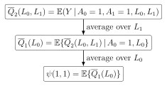
Longitudinal g-computation as backward nested averaging.

58.3 General \(K\)-Timepoint Formula

For a fixed regime \(\overline{a}=(a_0,\ldots,a_K)\), define \[\overline{Q}_{K+1}(\overline{L}_K) = \mathbb{E}(Y\,\vert\,\overline{A}_K=\overline{a}_K,\overline{L}_K).\] Then recursively define, for \(k=K,K-1,\ldots,1\), \[\overline{Q}_k(\overline{L}_{k-1}) = \mathbb{E}\{\overline{Q}_{k+1}(\overline{L}_k) \,\vert\,\overline{A}_{k-1}=\overline{a}_{k-1},\overline{L}_{k-1}\}.\] The target mean is \[\psi(\overline{a})=\mathbb{E}\{\overline{Q}_1(L_0)\}.\]

Equivalently, the formula can be displayed as nested expectations: \[\mathbb{E}\{Y(\overline{a})\} = \mathbb{E}\left[ \mathbb{E}\left[ \cdots \mathbb{E}\left[ \mathbb{E}(Y\,\vert\,\overline{A}_K=\overline{a}_K,\overline{L}_K) \,\vert\,\overline{A}_{K-1}=\overline{a}_{K-1},\overline{L}_{K-1} \right] \cdots \,\vert\,A_0=a_0,L_0 \right]\right].\]

58.4 Sequential Outcome Regressions

The functions \(\overline{Q}_{K+1},\overline{Q}_K,\ldots,\overline{Q}_1\) are called sequential outcome regressions. They are not all regressions of \(Y\). Only \(\overline{Q}_{K+1}\) is the conditional mean of the observed outcome. The earlier regressions use later predicted values as pseudo-outcomes.

For \(K=1\), the sequence is: \[\overline{Q}_2(L_0,L_1)=\mathbb{E}(Y\,\vert\,A_0=a_0,A_1=a_1,L_0,L_1),\] \[\overline{Q}_1(L_0)=\mathbb{E}\{\overline{Q}_2(L_0,L_1)\,\vert\,A_0=a_0,L_0\},\] \[\psi(a_0,a_1)=\mathbb{E}\{\overline{Q}_1(L_0)\}.\]

58.5 Interpretation of Nested Expectations

Each expectation performs one of two tasks. First, it replaces the observed treatment assignment with the regime value. Second, it averages over covariates that would naturally arise after earlier parts of the regime.

For the regime \((1,1)\), the inner regression asks: among people who received treatment at both times and had a given covariate history, what was the mean outcome? The next regression asks: among people who received treatment at time 0 and had a given \(L_0\), what covariate histories \(L_1\) occurred, and what outcomes would those histories imply if treatment also occurred at time 1? The final average transports these predicted means to the baseline target population.

Key Idea

Longitudinal g-computation is standardization over time. It standardizes the final outcome regression over the sequence of covariate distributions generated under the intervention history.

Lecture 8.4. Longitudinal IPTW Formula

59.1 Generalized Propensity Scores

For a point treatment, the propensity score is the conditional probability of receiving the observed or target treatment. In a longitudinal study, there is a time-specific treatment mechanism at every decision time.

Definition 59.1 (Generalized propensity score). For a binary treatment and fixed regime \(\overline{a}=(a_0,\ldots,a_K)\), define \[g_k(a_k\,\vert\,\overline{l}_k,\overline{a}_{k-1}) = \mathbb{P}(A_k=a_k\,\vert\,\overline{L}_k=\overline{l}_k,\overline{A}_{k-1}=\overline{a}_{k-1}).\] For the always-treated regime, write \[g_k(\overline{l}_k) = \mathbb{P}(A_k=1\,\vert\,\overline{L}_k=\overline{l}_k,\overline{A}_{k-1}=\mathbf{1}_k).\]

The time-specific propensity score is local: it concerns the treatment decision at time \(k\) among individuals whose previous treatment history is compatible with the regime.

59.2 Composite Treatment Probabilities

The probability of receiving an entire treatment profile is the product of the time-specific probabilities. For regime \(\overline{a}\) define \[\overline{g}_K(\overline{L}_K) = \prod_{k=0}^K g_k(a_k\,\vert\,\overline{L}_k,\overline{A}_{k-1}=\overline{a}_{k-1}).\] For the always-treated regime this is \[\overline{g}_K(\overline{L}_K) = g_0(L_0)g_1(\overline{L}_1)\cdots g_K(\overline{L}_K).\]

This product is the probability that a person with the realized covariate history would follow the regime through all treatment times, under the observed treatment mechanism.

59.3 Treatment-Regime Weights

The inverse probability weight for a regime \(\overline{a}\) is \[H_{\overline{a}} = \frac{\mathbb{1}(\overline{A}_K=\overline{a}_K)}{\overline{g}_K(\overline{L}_K)}.\] For the always-treated regime, \[H_{\mathbf{1}} = \frac{A_0A_1\cdots A_K} {g_0(L_0)g_1(\overline{L}_1)\cdots g_K(\overline{L}_K)}.\]

The numerator selects individuals whose observed treatment history matches the regime. The denominator upweights those individuals by the inverse probability of observing that full history.

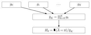
Longitudinal IPTW uses the product of time-specific treatment probabilities.

59.4 IPTW Identification for Treatment Profiles

Identification Result

Under consistency, sequential exchangeability, and longitudinal positivity, \[\mathbb{E}\{Y(\overline{a})\} = \mathbb{E}\left[ \frac{\mathbb{1}(\overline{A}_K=\overline{a}_K)} {\prod_{k=0}^K g_k(a_k\,\vert\,\overline{L}_k,\overline{A}_{k-1}=\overline{a}_{k-1})} Y \right].\] For the always-treated regime, \[\mathbb{E}\{Y(1,\ldots,1)\} = \mathbb{E}\left[ \frac{A_0A_1\cdots A_K} {g_0(L_0)g_1(\overline{L}_1)\cdots g_K(\overline{L}_K)} Y \right].\]

The formula creates a pseudo-population in which following the regime is no longer associated with measured history. Individuals with rare regime-compatible histories receive larger weights because they represent many similar individuals who did not follow the regime.

59.5 Positivity Problems Over Time

Longitudinal weights can become unstable quickly. If \(K=5\) and each time-specific probability equals \(0.5\), then the composite probability is \(0.5^6=0.015625\). The corresponding weight is \(64\) for an individual who follows the whole regime. If some probabilities are smaller, weights can be much larger.

There are two kinds of positivity problems:

Structural violations: a treatment sequence is impossible for some history, such as a contraindicated drug after severe toxicity.
Practical violations: the sequence is possible in principle but rarely observed in the sample.

Both problems are more common as the number of treatment times grows.

59.6 Equivalence with G-Computation

The IPTW and g-computation formulas identify the same counterfactual mean. The equivalence follows by repeated use of iterated expectation.

For the always-treated regime, let \[\overline{Q}_{K+1}(\overline{L}_K)=\mathbb{E}(Y\,\vert\,\overline{A}_K=\mathbf{1}_{K+1},\overline{L}_K).\] Then \[\begin{aligned} &\mathbb{E}\left[ \frac{A_0\cdots A_K}{g_0(\overline{L}_0)\cdots g_K(\overline{L}_K)}Y \right] \\ &= \mathbb{E}\left[ \frac{A_0\cdots A_K}{g_0(\overline{L}_0)\cdots g_K(\overline{L}_K)} \mathbb{E}(Y\,\vert\,\overline{L}_K,\overline{A}_K) \right] \\ &= \mathbb{E}\left[ \frac{A_0\cdots A_K}{g_0(\overline{L}_0)\cdots g_K(\overline{L}_K)} \overline{Q}_{K+1}(\overline{L}_K) \right]. \end{aligned}\] Now condition on \(\overline{L}_K,\overline{A}_{K-1}\). Since \[\mathbb{E}(A_K\,\vert\,\overline{L}_K,\overline{A}_{K-1}=\mathbf{1}_K)=g_K(\overline{L}_K),\] the factor \(A_K/g_K(\overline{L}_K)\) averages to one among those compatible with the past regime. Therefore the last expression becomes \[\mathbb{E}\left[ \frac{A_0\cdots A_{K-1}}{g_0(\overline{L}_0)\cdots g_{K-1}(\overline{L}_{K-1})} \mathbb{E}\{\overline{Q}_{K+1}(\overline{L}_K)\,\vert\,\overline{L}_{K-1},\overline{A}_{K-1}=\mathbf{1}_K\} \right].\] The conditional expectation is \(\overline{Q}_K(\overline{L}_{K-1})\). Repeating the same argument removes \(A_{K-1}/g_{K-1}\), then \(A_{K-2}/g_{K-2}\), and so on, yielding \[\mathbb{E}\{\overline{Q}_1(L_0)\},\] which is the g-computation formula.

Key Idea

IPTW and g-computation are two representations of the same identifying functional. G-computation integrates outcome regressions forward through the covariate process; IPTW reweights observed regime followers to represent the target population.

Lecture 8.5. Failure of Naive Regression

60.1 Regression Coefficients in Single-Timepoint Settings

Even in a point-treatment setting, a regression coefficient is not automatically an average treatment effect. Suppose \[\mathbb{E}(Y\,\vert\,A=a,W=w)=\beta_0+\beta_1 a+\beta_2 w.\] Then \[\mathbb{E}(Y\,\vert\,A=1,W=w)-\mathbb{E}(Y\,\vert\,A=0,W=w)=\beta_1\] for every \(w\), and the standardized mean difference is also \(\beta_1\): \[\mathbb{E}\{\mathbb{E}(Y\,\vert\,A=1,W)-\mathbb{E}(Y\,\vert\,A=0,W)\}=\beta_1.\] This special equality depends on the linear model and the absence of treatment effect modification by \(W\).

60.2 Linear Models Without Interactions

When a linear model has no interaction between treatment and covariates, the treatment coefficient is a constant conditional mean contrast. Under the usual identification assumptions, it can equal the g-computation estimate of the ATE. This is a special case, not a general rule.

60.3 Linear Models With Interactions

If the conditional mean includes an interaction, \[\mathbb{E}(Y\,\vert\,A=a,W=w)=\beta_0+\beta_1a+\beta_2w+\beta_3aw,\] then the conditional contrast is \[\mathbb{E}(Y\,\vert\,A=1,W=w)-\mathbb{E}(Y\,\vert\,A=0,W=w)=\beta_1+\beta_3w.\] The marginal standardized contrast is \[\mathbb{E}(\beta_1+\beta_3W)=\beta_1+\beta_3\mathbb{E}(W).\] Thus \(\beta_1\) is the conditional contrast at \(W=0\), not the average treatment effect unless \(\mathbb{E}(W)=0\) or \(\beta_3=0\).

60.4 Logistic Models

For binary outcomes, logistic regression is nonlinear: \[\mathbb{E}(Y\,\vert\,A=a,W=w)=\mathop{\mathrm{expit}}(\beta_0+\beta_1a+\beta_2w).\] The risk difference at covariate value \(w\) is \[\mathop{\mathrm{expit}}(\beta_0+\beta_1+\beta_2w)-\mathop{\mathrm{expit}}(\beta_0+\beta_2w),\] and the marginal risk difference is \[\mathbb{E}\left[ \mathop{\mathrm{expit}}(\beta_0+\beta_1+\beta_2W)-\mathop{\mathrm{expit}}(\beta_0+\beta_2W) \right].\] The coefficient \(\beta_1\) is a conditional log-odds ratio parameter, not a risk difference and not a marginal ATE.

60.5 Time-Varying Confounder Feedback

Longitudinal settings introduce a deeper problem. Consider \[L_0 \rightarrow A_0 \rightarrow L_1 \rightarrow A_1 \rightarrow Y,\] where \(L_1\) also affects \(Y\). A regression of \(Y\) on \(A_0,L_1,A_1\) conditions on \(L_1\). This may be useful for estimating the effect of \(A_1\), because \(L_1\) confounds the \(A_1\)–\(Y\) relation. But it blocks part of the effect of \(A_0\) on \(Y\) that operates through \(L_1\).

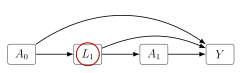
Conditioning on \(L_1\) can block the mediated path from \(A_0\) to \(Y\) while controlling confounding for \(A_1\).

60.6 A Numerical Data-Generating Example

Suppose \[A_0\sim \operatorname{Bernoulli}(0.5),\] \[L_1\,\vert\,A_0=a_0 \sim N(1+a_0,1),\] \[A_1\,\vert\,L_1=l_1,A_0=a_0 \sim \operatorname{Bernoulli}\{\mathop{\mathrm{expit}}(-1+l_1+a_0)\},\] and \[Y\,\vert\,A_1=a_1,L_1=l_1,A_0=a_0 \sim N(1+a_1+2l_1,1).\] The mean outcome regression does not contain \(A_0\) directly. Nevertheless, \(A_0\) has a causal effect because it shifts \(L_1\), and \(L_1\) affects \(Y\).

Using g-computation, \[\begin{aligned} \mathbb{E}\{Y(1,1)\} &=\mathbb{E}\{\mathbb{E}(Y\,\vert\,A_1=1,L_1,A_0=1)\,\vert\,A_0=1\}\\ &=\mathbb{E}(2+2L_1\,\vert\,A_0=1)=2+2(2)=6, \end{aligned}\] because \(\mathbb{E}(L_1\,\vert\,A_0=1)=2\). Similarly, \[\mathbb{E}\{Y(1,0)\}=5,\qquad \mathbb{E}\{Y(0,1)\}=4,\qquad \mathbb{E}\{Y(0,0)\}=3.\] Therefore the effect of changing \(A_0\) from 0 to 1 while holding \(A_1=1\) is \[\mathbb{E}\{Y(1,1)-Y(0,1)\}=2.\]

Now fit the correctly specified conditional mean regression \[\mathbb{E}(Y\,\vert\,A_1,L_1,A_0)=1+A_1+2L_1+0\cdot A_0.\] The coefficient on \(A_0\) is zero because the regression conditions on \(L_1\). Reading the \(A_0\) coefficient as the causal effect of baseline treatment would therefore be wrong.

60.7 Blocking Causal Pathways by Conditioning on Intermediates

The problem is not that regression is useless. The problem is using one conditional regression as if it were the causal estimand. Sequential g-computation uses regressions carefully: it conditions on \(L_1\) in the final outcome regression and then averages over the distribution of \(L_1\) that would arise under each baseline treatment. A naive regression coefficient conditions on \(L_1\) and stops there.

Key Idea

In longitudinal studies, the same covariate can be a confounder for later treatment and a mediator for earlier treatment. Ordinary regression adjustment cannot generally handle this feedback by reading off coefficients.

Lecture 8.6. IPTW Estimation for Time-Varying Interventions

61.1 Estimating Time-Specific Propensity Scores

The longitudinal IPTW identification formula suggests a direct estimator. For a fixed regime \(\overline{a}\), estimate each treatment mechanism \[g_k(a_k\,\vert\,\overline{L}_k,\overline{A}_{k-1}=\overline{a}_{k-1})\] and then average the weighted outcomes among individuals whose observed treatment history matches the regime.

For two treatment times and binary treatments, estimate \[g_0(a_0\,\vert\,L_0)=\mathbb{P}(A_0=a_0\,\vert\,L_0),\] and \[g_1(a_1\,\vert\,L_0,A_0=a_0,L_1) = \mathbb{P}(A_1=a_1\,\vert\,L_0,A_0=a_0,L_1).\] The models for these probabilities may be logistic regressions, Super Learner fits, or other binary regression estimators.

61.2 Constructing Cumulative Weights

For subject \(i\), define the estimated regime probability \[\overline{g}_{n,K,i}(\overline{a}) = \prod_{k=0}^K g_{n,k}(a_k\,\vert\,\overline{L}_{k,i},\overline{A}_{k-1,i}=\overline{a}_{k-1}).\] The estimated weight is \[H_{n,i}(\overline{a}) = \frac{\mathbb{1}(\overline{A}_{K,i}=\overline{a}_K)}{\overline{g}_{n,K,i}(\overline{a})}.\]

Estimation Notes

The IPTW estimator of the counterfactual mean under regime \(\overline{a}\) is \[\psi_{n,\operatorname{IPTW}}(\overline{a}) = \frac{1}{n}\sum_{i=1}^n H_{n,i}(\overline{a})Y_i.\] An ATE comparing regimes \(\overline{a}\) and \(\overline{a}'\) is estimated by \[\psi_{n,\operatorname{IPTW}}(\overline{a})-\psi_{n,\operatorname{IPTW}}(\overline{a}').\]

Some analysts use stabilized weights to reduce variance. For a static regime, a stabilized weight has a numerator that models the probability of the treatment history using less covariate information, for example \[\prod_{k=0}^K \mathbb{P}(A_k=a_k\,\vert\,\overline{A}_{k-1}=\overline{a}_{k-1}),\] divided by the full denominator. Stabilization changes the variance properties, but the denominator is still the part that removes measured confounding.

61.3 Estimating Counterfactual Means

For \(K=1\) and regime \((1,1)\), \[\psi_{n,\operatorname{IPTW}}(1,1) = \frac{1}{n}\sum_{i=1}^n \frac{\mathbb{1}(A_{0i}=1,A_{1i}=1)} {g_{n,0}(1\,\vert\,L_{0i}) g_{n,1}(1\,\vert\,L_{0i},A_0=1,L_{1i})} Y_i.\] For regime \((1,0)\), \[\psi_{n,\operatorname{IPTW}}(1,0) = \frac{1}{n}\sum_{i=1}^n \frac{\mathbb{1}(A_{0i}=1,A_{1i}=0)} {g_{n,0}(1\,\vert\,L_{0i}) \{1-g_{n,1}(1\,\vert\,L_{0i},A_0=1,L_{1i})\}} Y_i.\] The same pattern applies to \((0,1)\) and \((0,0)\), with the appropriate probabilities in the denominator.

61.4 R Implementation

The following code implements the two-timepoint estimator in a simulated data set with variables ‘A0‘, ‘L1‘, ‘A1‘, and ‘Y‘. The treatment at time 0 is randomized in this example, so the first propensity model is intercept-only.

# time-0 treatment mechanism
ps0 <- glm(A0 ~ 1, family = binomial())
g_0 <- predict(ps0, type = "response")

# time-1 treatment mechanism
ps1 <- glm(A1 ~ L1 + A0, family = binomial())

# P(A1 = 1 | A0 = 1, L1 = L1_i)
g_1_A0_1 <- predict(
  ps1,
  newdata = data.frame(A0 = 1, L1 = L1),
  type = "response"
)

# P(A1 = 1 | A0 = 0, L1 = L1_i)
g_1_A0_0 <- predict(
  ps1,
  newdata = data.frame(A0 = 0, L1 = L1),
  type = "response"
)

EY_11 <- mean((A0 == 1 & A1 == 1) / (g_0 * g_1_A0_1) * Y)
EY_10 <- mean((A0 == 1 & A1 == 0) / (g_0 * (1 - g_1_A0_1)) * Y)
EY_01 <- mean((A0 == 0 & A1 == 1) / ((1 - g_0) * g_1_A0_0) * Y)
EY_00 <- mean((A0 == 0 & A1 == 0) / ((1 - g_0) * (1 - g_1_A0_0)) * Y)

ate_11_vs_00 <- EY_11 - EY_00

61.5 Simulated Examples

In the data-generating example from Section 60, the true counterfactual means are \[\mathbb{E}\{Y(1,1)\}=6,\quad \mathbb{E}\{Y(1,0)\}=5,\quad \mathbb{E}\{Y(0,1)\}=4,\quad \mathbb{E}\{Y(0,0)\}=3.\] If the propensity score models are correctly specified and the sample is large, the IPTW estimates should be close to these values. Discrepancies in finite samples arise from random error, propensity score estimation error, and weight instability.

61.6 Diagnosing Extreme Weights

Because longitudinal weights multiply inverse probabilities, diagnostics are essential. At a minimum, inspect:

summaries of each time-specific propensity score;
summaries of the cumulative denominator \(\overline{g}_{n,K}\);
summaries of the final weights \(H_{n,i}(\overline{a})\);
the number of individuals who follow each regime;
whether large weights are concentrated in clinically unusual histories.

w_11 <- (A0 == 1 & A1 == 1) / (g_0 * g_1_A0_1)

summary(g_0)
summary(g_1_A0_1)
summary(w_11)
quantile(w_11, probs = c(.5, .9, .95, .99, 1))
mean(A0 == 1 & A1 == 1)

Large weights do not automatically imply bias, but they indicate that the estimate depends heavily on a small number of observations. Truncating weights can reduce variance but changes the estimand or introduces bias, so it should be reported as a sensitivity analysis rather than hidden as a default.

Key Idea

Longitudinal IPTW is simple to compute once time-specific propensity scores are available, but it can be highly variable because a full treatment history may be rare even when each individual treatment decision is not rare.

Lecture 8.7. Sequential Regression G-Computation

62.1 Backward Recursive Regressions

Sequential regression is an implementation of the longitudinal g-computation formula that avoids explicitly estimating the full conditional distribution of each time-varying covariate. Instead, it works backward from the final outcome.

For \(K=1\) and regime \((a_0,a_1)\): \[\overline{Q}_2(L_0,L_1)=\mathbb{E}(Y\,\vert\,A_0=a_0,A_1=a_1,L_0,L_1),\] \[\overline{Q}_1(L_0)=\mathbb{E}\{\overline{Q}_2(L_0,L_1)\,\vert\,A_0=a_0,L_0\},\] \[\psi(a_0,a_1)=\mathbb{E}\{\overline{Q}_1(L_0)\}.\] Sequential regression estimates \(\overline{Q}_2\), predicts it for all individuals, then uses those predictions as the outcome in a regression for \(\overline{Q}_1\) among individuals with \(A_0=a_0\).

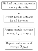
Sequential regression implements g-computation by backward recursion.

62.2 Pseudo-Outcomes

A pseudo-outcome is a fitted value from a later regression that becomes the outcome for an earlier regression. In the two-timepoint case:

Fit a regression for \(Y\) among those with \(A_0=a_0,A_1=a_1\).
Predict \(\overline{Q}_{2,n}(L_{0i},L_{1i})\) for every individual.
Among those with \(A_0=a_0\), regress \(\overline{Q}_{2,n}(L_{0i},L_{1i})\) on \(L_{0i}\).
Predict \(\overline{Q}_{1,n}(L_{0i})\) for every individual.
Average these predictions.

This is a regression-based way to perform the integration over \(L_1\) required by the g-computation formula.

62.3 Binary Time-Varying Confounders

If \(L_1\) is binary or low-dimensional discrete, one can also implement g-computation by explicitly summing over possible \(L_1\) values: \[\overline{Q}_1(L_0) = \sum_{l_1} \overline{Q}_2(L_0,l_1) \mathbb{P}(L_1=l_1\,\vert\,A_0=a_0,L_0).\] For binary \(L_1\), \[\begin{aligned} \overline{Q}_1(L_0) &= \overline{Q}_2(L_0,1)\mathbb{P}(L_1=1\,\vert\,A_0=a_0,L_0)\\ &\quad+ \overline{Q}_2(L_0,0)\mathbb{P}(L_1=0\,\vert\,A_0=a_0,L_0). \end{aligned}\] This approach is transparent, but it becomes difficult when time-varying covariates are continuous or high-dimensional.

62.4 Estimating \(\overline{Q}_{K+1},\overline{Q}_K,\ldots,\overline{Q}_1\)

For a general fixed regime \(\overline{a}\), sequential regression proceeds as follows:

Estimation Notes

Estimate \[\overline{Q}_{K+1}(\overline{L}_K)= \mathbb{E}(Y\,\vert\,\overline{A}_K=\overline{a}_K,\overline{L}_K)\] using observations with \(\overline{A}_K=\overline{a}_K\).
Predict \(\overline{Q}_{K+1,n}(\overline{L}_{K,i})\) for all individuals.
For \(k=K,K-1,\ldots,1\), estimate \[\overline{Q}_k(\overline{L}_{k-1})= \mathbb{E}\{\overline{Q}_{k+1}(\overline{L}_k)\,\vert\, \overline{A}_{k-1}=\overline{a}_{k-1},\overline{L}_{k-1}\}\] by regressing the current pseudo-outcome on \(\overline{L}_{k-1}\) among those with \(\overline{A}_{k-1}=\overline{a}_{k-1}\).
Estimate \[\psi(\overline{a})=\frac{1}{n}\sum_{i=1}^n \overline{Q}_{1,n}(L_{0i}).\]

62.5 R Implementation

For two treatment times and regime \((1,1)\):

full_data <- data.frame(L0 = L0, A0 = A0, L1 = L1, A1 = A1, Y = Y)

# Step 1: final outcome regression among regime followers
data_11 <- subset(full_data, A0 == 1 & A1 == 1)
fit_Q2 <- glm(Y ~ L0 + L1, data = data_11)

# Step 2: predict Q2 for everyone at their observed L0, L1
full_data$Q2n <- predict(fit_Q2, newdata = full_data, type = "response")

# Step 3: regress the pseudo-outcome among those with A0 = 1
data_1 <- subset(full_data, A0 == 1)
fit_Q1 <- glm(Q2n ~ L0, data = data_1)

# Step 4: predict Q1 for everyone and average
full_data$Q1n <- predict(fit_Q1, newdata = full_data, type = "response")
psi_11 <- mean(full_data$Q1n)

If the outcome is binary, logistic regression may be used for both steps:

fit_Q2 <- glm(Y ~ L0 + L1, data = data_11, family = binomial())
full_data$Q2n <- predict(fit_Q2, newdata = full_data, type = "response")

fit_Q1 <- glm(Q2n ~ L0, data = data_1, family = binomial())
full_data$Q1n <- predict(fit_Q1, newdata = full_data, type = "response")
psi_11 <- mean(full_data$Q1n)

62.6 Comparing With IPTW

Sequential regression and IPTW estimate the same counterfactual mean under the same identification assumptions, but they rely on different nuisance functions. Sequential regression relies on the outcome regression sequence \(\overline{Q}_{K+1},\ldots,\overline{Q}_1\). IPTW relies on the treatment mechanism sequence \(g_0,\ldots,g_K\).

Sequential regression often has lower variance because it does not use inverse probability weights. However, it can be biased if the sequential outcome regressions are misspecified. IPTW may be more robust to outcome model misspecification but can be unstable under near-positivity violations.

Key Idea

Sequential regression turns nested expectations into a sequence of prediction problems. At each step, the outcome is the predicted counterfactual mean from the next later step.

Lecture 8.8. Doubly Robust Longitudinal Estimation

63.1 Longitudinal AIPTW

Longitudinal augmented inverse probability weighting combines the sequential outcome-regression representation with the longitudinal weighting representation. For the always-treated regime, define \[\overline{g}_{j,n}(\overline{L}_j)=\prod_{m=0}^j g_{m,n}(\overline{L}_m),\] and let \(\overline{Q}_{j,n}\) estimate the sequential outcome regressions from Section 58. The baseline plug-in part is the sequential g-computation estimate \[\frac{1}{n}\sum_{i=1}^n \overline{Q}_{1,n}(L_{0i}).\] The weighted residual corrections are applied after this baseline averaging. For \(j=0,\ldots,K-1\), define \[\Delta_{ji} = \overline{Q}_{j+2,n}(\overline{L}_{j+1,i}) - \overline{Q}_{j+1,n}(\overline{L}_{j,i}),\] and define the final residual as \[\Delta_{Ki} = Y_i-\overline{Q}_{K+1,n}(\overline{L}_{K,i}).\] The longitudinal AIPTW estimator can then be written as \[\psi_{n,\operatorname{AIPTW}} = \frac{1}{n}\sum_{i=1}^n \overline{Q}_{1,n}(L_{0i}) + \frac{1}{n}\sum_{i=1}^n \sum_{j=0}^K \frac{A_{0i}\cdots A_{ji}}{\overline{g}_{j,n}(\overline{L}_{j,i})} \Delta_{ji},\] with the convention that \(\overline{Q}_{K+1,n}(\overline{L}_K)\) is the final outcome regression. The baseline plug-in term is not weighted; only the residual corrections are weighted by regime-following inverse probabilities.

For \(K=1\) and regime \((1,1)\), this becomes \[\begin{aligned} \psi_{n,\operatorname{AIPTW}} &= \frac{1}{n}\sum_{i=1}^n \overline{Q}_{1,n}(L_{0i})\\ &\quad+ \frac{1}{n}\sum_{i=1}^n \frac{A_{0i}}{g_{0,n}(L_{0i})} \{\overline{Q}_{2,n}(L_{0i},L_{1i})-\overline{Q}_{1,n}(L_{0i})\}\\ &\quad+ \frac{1}{n}\sum_{i=1}^n \frac{A_{0i}A_{1i}}{g_{0,n}(L_{0i})g_{1,n}(\overline{L}_{1i})} \{Y_i-\overline{Q}_{2,n}(L_{0i},L_{1i})\}. \end{aligned}\] The first line is sequential g-computation. The second and third lines are weighted residual corrections at time 0 and time 1.

63.2 Nuisance Functions Over Time

Longitudinal doubly robust estimation uses two nuisance sequences: \[\overline{Q}=(\overline{Q}_1,\ldots,\overline{Q}_{K+1}), \qquad g=(g_0,\ldots,g_K).\] The \(\overline{Q}\) sequence describes outcome and pseudo-outcome regressions. The \(g\) sequence describes the treatment process. The estimator uses both because each sequence can help correct errors in the other.

63.3 Double Robustness in Multi-Timepoint Settings

Definition 63.1 (Longitudinal double robustness). A longitudinal estimator is doubly robust if it consistently estimates \(\mathbb{E}\{Y(\overline{a})\}\) when either the required outcome-regression sequence is consistently estimated or the required treatment-mechanism sequence is consistently estimated, under the other identification assumptions.

For multiple time points, there are also mixed robustness patterns. Roughly, the estimator can remain consistent when the treatment mechanism is consistently estimated for earlier parts of the process and the outcome regressions are consistently estimated for later parts. The exact statement depends on the recursive representation of the estimator, but the practical message is that longitudinal AIPTW has more robustness than pure g-computation or pure IPTW. Mixed robustness is not an arbitrary mix-and-match property: the exact combinations of correctly estimated \(\overline{Q}\)- and \(g\)-components that yield consistency depend on the recursive estimator and its indexing.

63.4 Correct \(\overline{Q}\)-Sequence

If the sequential outcome regressions are consistently estimated, then the g-computation component already converges to the target: \[\frac{1}{n}\sum_{i=1}^n\overline{Q}_{1,n}(L_{0i}) \rightarrow \mathbb{E}\{Y(\overline{a})\}.\] The weighted residual augmentation terms have mean approximately zero because the residuals \[\Delta_{ji}\] are centered correctly given the earlier histories. Thus the estimator remains consistent even if the propensity scores are not consistently estimated, provided the weights are well behaved.

63.5 Correct \(g\)-Sequence

If the treatment mechanisms are consistently estimated, the weighted residual terms correct bias in the outcome regressions. The intuition is the same as in the point-treatment AIPTW estimator. The inverse probability weights make the observed regime-compatible histories representative of the target population, and the residual terms repair the g-computation plug-in estimate.

For \(K=1\), if \(g_{0,n}\) and \(g_{1,n}\) converge to the true treatment mechanisms, then the weighted residuals at the two stages remove the drift caused by incorrect \(\overline{Q}_{1,n}\) and \(\overline{Q}_{2,n}\).

63.6 Mixed Robustness Patterns Over Time

With many treatment times, robustness can be more nuanced. For example, an estimator may be consistent if:

the treatment mechanisms are correct through early time points, and
the outcome regressions are correct from a later time point onward.

This occurs because backward recursion only needs enough correct information to bridge each step between the final outcome and baseline. However, this should not be interpreted as permission to fit careless models. A misspecified nuisance function can still harm finite-sample performance, inflate variance, and damage inference. The valid mixed-robustness patterns are estimator-specific, not arbitrary choices of some correct \(g\) terms and some correct \(\overline{Q}\) terms.

Estimation Notes

The longitudinal AIPTW workflow is:

Fit all time-specific propensity score models \(g_{0,n},\ldots,g_{K,n}\).
Fit the sequential outcome regressions \(\overline{Q}_{K+1,n},\ldots,\overline{Q}_{1,n}\).
Compute the g-computation plug-in estimate \(n^{-1}\sum_i\overline{Q}_{1,n}(L_{0i})\).
Add weighted residual corrections at each time point.
Estimate uncertainty using the empirical variance of the estimated influence-function contributions, with caution when nuisance fits are highly adaptive.

Key Idea

Longitudinal AIPTW corrects sequential g-computation by adding weighted residuals at every treatment time. Its robustness comes from using both the outcome process and the treatment process.

Lecture 8.9. Longitudinal TMLE

64.1 Sequential TMLE Algorithm

Targeted minimum loss-based estimation (TMLE) modifies sequential g-computation so that the final estimator remains a plug-in estimator while also solving bias-correction equations related to the efficient influence function. In longitudinal settings, TMLE proceeds backward through time, just like sequential regression, but inserts a targeting step after each outcome regression.

For the always-treated regime, the algorithm has the following structure:

Estimate the final outcome regression \(\overline{Q}_{K+1,n}(\overline{L}_K)=\mathbb{E}_n(Y\,\vert\,\overline{A}_K=\mathbf{1},\overline{L}_K)\).
Target this regression using a clever covariate based on \(1/\overline{g}_{K,n}\), producing \(\overline{Q}_{K+1,n}^*\).
Regress \(\overline{Q}_{K+1,n}^*\) on earlier history among individuals who followed the regime through time \(K-1\), producing \(\overline{Q}_{K,n}\).
Target \(\overline{Q}_{K,n}\) using the clever covariate based on \(1/\overline{g}_{K-1,n}\), producing \(\overline{Q}_{K,n}^*\).
Continue backward until \(\overline{Q}_{1,n}^*\) is obtained.
Estimate the target mean by \[\psi_{n,\operatorname{TMLE}}=\frac{1}{n}\sum_{i=1}^n \overline{Q}_{1,n}^*(L_{0i}).\]

64.3 Clever Covariates

For two treatment times and regime \((1,1)\), the final outcome regression is \[\overline{Q}_{2,n}(L_0,L_1)\approx \mathbb{E}(Y\,\vert\,A_0=1,A_1=1,L_0,L_1).\] The clever covariate for targeting this regression is \[H_{2,n}=\frac{\mathbb{1}(A_0=1,A_1=1)} {g_{0,n}(L_0)g_{1,n}(\overline{L}_1)}.\] A logistic fluctuation fits \[\mathop{\mathrm{logit}}\{\overline{Q}_{2,n}^*(L_0,L_1)\} = \mathop{\mathrm{logit}}\{\overline{Q}_{2,n}(L_0,L_1)\} +\hat\epsilon_2 H_{2,n}.\] The next regression estimates \[\overline{Q}_{1,n}(L_0)\approx \mathbb{E}\{\overline{Q}_{2,n}^*(L_0,L_1)\,\vert\,A_0=1,L_0\},\] and its clever covariate is \[H_{1,n}=\frac{\mathbb{1}(A_0=1)}{g_{0,n}(L_0)}.\] The update is \[\mathop{\mathrm{logit}}\{\overline{Q}_{1,n}^*(L_0)\} = \mathop{\mathrm{logit}}\{\overline{Q}_{1,n}(L_0)\}+\hat\epsilon_1H_{1,n}.\]

64.4 Final Plug-In Estimate

The final estimate is \[\psi_{n,\operatorname{TMLE}}(1,1)=\frac{1}{n}\sum_{i=1}^n\overline{Q}_{1,n}^*(L_{0i}).\] It is a plug-in estimator because it is the empirical mean of an updated counterfactual outcome regression. For binary outcomes, this guarantees that the estimate lies in \([0,1]\), unlike some weighted estimators that can behave poorly in small samples.

64.5 TMLE Implementation in R

The following sketch shows the two-timepoint binary-outcome implementation.

# propensity scores
ps0_fit <- glm(A0 ~ L0, family = binomial())
ps1_fit <- glm(A1 ~ L0 + A0 + L1, family = binomial())

g_0 <- predict(ps0_fit, type = "response")
g_1 <- predict(
  ps1_fit,
  newdata = data.frame(L0 = L0, A0 = 1, L1 = L1),
  type = "response"
)

# initial Q2
or2_fit <- glm(Y ~ A0 + A1 + L0 + L1, family = binomial())
Q2_obs <- predict(or2_fit, type = "response")
Q2_11 <- predict(
  or2_fit,
  newdata = data.frame(A0 = 1, A1 = 1, L0 = L0, L1 = L1),
  type = "response"
)

# target Q2
H2 <- (A0 == 1 & A1 == 1) / (g_0 * g_1)
eps2_fit <- glm(
  Y ~ -1 + offset(qlogis(Q2_obs)) + H2,
  family = binomial()
)
Q2_11_star <- plogis(qlogis(Q2_11) + coef(eps2_fit)["H2"] / (g_0 * g_1))

# initial Q1
or1_fit <- glm(Q2_11_star ~ A0 * L0, family = binomial())
Q1_obs <- predict(or1_fit, type = "response")
Q1_1 <- predict(
  or1_fit,
  newdata = data.frame(A0 = 1, L0 = L0),
  type = "response"
)

# target Q1
H1 <- (A0 == 1) / g_0
eps1_fit <- glm(
  Q2_11_star ~ -1 + offset(qlogis(Q1_obs)) + H1,
  family = binomial()
)
Q1_1_star <- plogis(qlogis(Q1_1) + coef(eps1_fit)["H1"] / g_0)

psi_tmle <- mean(Q1_1_star)

64.6 Relationship to Sequential Regression

Sequential regression estimates the nested g-computation formula and stops. Longitudinal TMLE follows the same backward structure, but after each regression it performs a targeted update using the propensity score sequence. This update is designed so that the empirical mean of the efficient influence-function component is close to zero.

Key Idea

Longitudinal TMLE is targeted sequential regression. It keeps the plug-in interpretation of g-computation while incorporating inverse-probability information through clever covariates.

Lecture 8.10. Time-to-Event and Competing Risks

65.1 Longitudinal Data With Event Times

Time-to-event data can be represented using the same longitudinal structure as time-varying treatments. Let \(T\) be the event time of interest and let \(C\) be a right-censoring time. The observed time is \[\widetilde T=\min(T,C),\] with event indicator \[\Delta=\mathbb{1}(T\le C).\] For causal questions, one often wants the counterfactual cumulative incidence \[\mathbb{P}\{T(a)\le t\}\] or its longitudinal analogue under a treatment or censoring intervention.

Discretize time into intervals \(1,\ldots,t\). Define \[L_j=\mathbb{1}(\text{event has occurred by time } j),\] and let \(A_j\) indicate remaining uncensored through the relevant interval. Then \[\mathbb{P}\{T(a)\le t\}=\mathbb{P}\{L_t(a)=1\}.\] The event process \(L_j\) is a counting process with an absorbing state: once \(L_j=1\), all later \(L_s\) for \(s>j\) must also equal 1.

65.2 Censoring

Right censoring can be viewed as a time-varying process that prevents later outcomes from being observed. If \(A_j=1\) denotes not being censored through time \(j\), then estimating a full-data event probability can be framed as estimating the outcome under the intervention \[A_1=A_2=\cdots=A_t=1,\] that is, the intervention that eliminates censoring.

Causal Assumption

Identification under censoring requires sequential exchangeability for the censoring process: \[L_t(\bar a) \perp\!\!\!\perp A_j \,\vert\,\overline{L}_j,\overline{A}_{j-1} \qquad j=1,\ldots,t.\] In words, among people with the same observed history, remaining uncensored is independent of the counterfactual event status that would be observed under the no-censoring intervention.

65.3 Sequential Regression for Survival Outcomes

Consider estimating \(\mathbb{P}\{L_3(1,1,1)=1\}\), the cumulative incidence by time 3 under no censoring. A sequential regression algorithm works backward:

Estimate \[\overline{Q}_3(\overline{L}_2)=\mathbb{E}(L_3\,\vert\,\overline{A}_3=\mathbf{1},\overline{L}_2).\] If \(L_2=1\), then \(\overline{Q}_3(\overline{L}_2)=1\) by the absorbing event structure. Therefore only histories with \(L_2=0\) require a regression model.
Build a pseudo-outcome \(\overline{Q}_{3,n}\) that equals 1 for those with \(L_2=1\) and equals the fitted probability for those with \(L_2=0\).
Estimate \[\overline{Q}_2(\overline{L}_1)=\mathbb{E}\{\overline{Q}_3(\overline{L}_2)\,\vert\,\overline{A}_2=\mathbf{1},\overline{L}_1\}.\] If \(L_1=1\), then \(\overline{Q}_2(\overline{L}_1)=1\).
Continue backward and average the final prediction over baseline covariates.

# L1, L2, L3 are indicators of event by times 1, 2, 3.
# A1, A2, A3 are indicators of remaining uncensored.

full_data$Q3n <- NA
full_data$Q3n[full_data$L2 == 1] <- 1

fit_data_Q3 <- subset(
  full_data,
  A1 == 1 & A2 == 1 & A3 == 1 & L2 == 0
)
fit_Q3 <- glm(L3 ~ L0, data = fit_data_Q3, family = binomial())

pred_data <- full_data[full_data$L2 == 0, ]
full_data$Q3n[full_data$L2 == 0] <-
  predict(fit_Q3, newdata = pred_data, type = "response")

full_data$Q2n <- NA
full_data$Q2n[full_data$L1 == 1] <- 1

fit_data_Q2 <- subset(full_data, A1 == 1 & A2 == 1 & L1 == 0)
fit_Q2 <- glm(Q3n ~ L0, data = fit_data_Q2, family = binomial())

pred_data <- full_data[full_data$L1 == 0, ]
full_data$Q2n[full_data$L1 == 0] <-
  predict(fit_Q2, newdata = pred_data, type = "response")

fit_data_Q1 <- subset(full_data, A1 == 1)
fit_Q1 <- glm(Q2n ~ L0, data = fit_data_Q1, family = binomial())
full_data$Q1n <- predict(fit_Q1, newdata = full_data, type = "response")

cuminc_3 <- mean(full_data$Q1n)

65.4 Competing Risks

In competing risks, the first event may be one of several types. Let \(J\in\{1,\ldots,m\}\) denote event type. The observed event indicator may take values \[\Delta=0 \text{ for censoring},\qquad \Delta=j \text{ for an event of type } j.\] For discrete time, define \[L_{kj}=\mathbb{1}(\text{event of type } j \text{ has occurred by time } k),\] and collect these into \[L_k=(L_{k1},\ldots,L_{km}).\] The type-\(j\) cumulative incidence is \[\mathbb{P}\{T(a)\le t,J(a)=j\}=\mathbb{P}\{L_{tj}(a)=1\}.\]

The absorbing structure is more restrictive than in the single-event case. If a type 1 event occurred by time \(k\), then type 1 remains occurred at all later times and no other first-event type can occur later. For two event types: \[L_{k1}=1 \Rightarrow L_{s1}=1,\ L_{s2}=0 \quad\text{for }s>k.\]

65.5 Counterfactual Cumulative Incidence

The counterfactual cumulative incidence under treatment or no censoring is a standard longitudinal counterfactual mean. The outcome is the event indicator by time \(t\), and the intervention may set treatment, censoring, or both.

For example, with no censoring through time \(t\), \[\psi_j(t)=\mathbb{E}\{L_{tj}(\mathbf{1})\} = \mathbb{P}\{T(\mathbf{1})\le t,J(\mathbf{1})=j\}.\] Contrasts of \(\psi_j(t)\) across treatment regimes are causal contrasts of cumulative incidence curves.

65.6 Practical Estimation Issues

Survival and competing-risk estimation require the analyst to respect deterministic history restrictions:

do not fit event regressions among people who already had the event when the outcome is already known;
set the pseudo-outcome to 1 after the target event has occurred;
set the pseudo-outcome to 0 after a competing first event has occurred when estimating the cumulative incidence of a different event type;
define censoring indicators carefully so that future outcomes are not used after censoring.

Key Idea

Time-to-event data become longitudinal data after discretization. The main extra work is enforcing the absorbing-state logic of event histories and, for competing risks, the mutually exclusive nature of first-event types.

Lecture 8.11. Dynamic Treatment Rules

66.1 Static vs Dynamic Regimes

A static regime assigns the same treatment sequence to everyone: \[\overline{a}=(a_0,\ldots,a_K).\] Examples are always treat, never treat, or treat at visits 0 and 1 only.

A dynamic regime assigns treatment according to observed history. It is a sequence of rules \[d=(d_0,\ldots,d_K),\] where \[A_k=d_k(\overline{L}_k,\overline{A}_{k-1}).\] The rule may depend on laboratory values, symptoms, adverse events, previous treatment, or other information available at time \(k\).

66.2 Rule-Based Interventions

Definition 66.1 (Dynamic treatment rule). A dynamic treatment rule is an intervention that sets treatment at each time to a deterministic or stochastic function of the individual’s observed history up to that time.

For example, in inflammatory bowel disease, a drug may be recommended only while liver function remains adequate: \[d_k(\overline{L}_k)= \begin{cases} 1, & \text{if recent liver function is adequate},\\ 0, & \text{otherwise}. \end{cases}\] This rule is more realistic than “always treat” if treatment is contraindicated after signs of liver damage.

66.3 Treatment Decisions Based on Evolving Covariates

Dynamic regimes are often clinically natural because real treatment decisions respond to evolving information. A rule might say:

continue chemotherapy if tumor response is adequate and toxicity is mild;
intensify antihypertensive therapy if blood pressure remains high;
stop a medication if a severe adverse event occurs;
initiate rescue therapy if symptoms cross a threshold.

A dynamic rule maps the evolving observed history into treatment decisions.

66.4 Counterfactual Outcomes Under Dynamic Rules

Let \(Y(d)\) denote the outcome that would be observed if treatment were assigned according to rule \(d\) at every time point. The causal mean under the rule is \[\psi(d)=\mathbb{E}\{Y(d)\}.\] A causal contrast between two rules is \[\psi(d)-\psi(d') = \mathbb{E}\{Y(d)\}-\mathbb{E}\{Y(d')\}.\]

The consistency assumption for a dynamic rule states that if an individual’s observed treatment history happens to agree with the rule at every time, then the observed outcome equals the counterfactual outcome under that rule: \[\text{if } A_k=d_k(\overline{L}_k,\overline{A}_{k-1})\text{ for all }k, \quad Y=Y(d).\]

66.5 Identification Extensions

Identification conditions are the dynamic-rule versions of the static-regime conditions. Sequential exchangeability becomes \[Y(d) \perp\!\!\!\perp A_k \,\vert\,\overline{L}_k,\overline{A}_{k-1}\] among histories compatible with the rule up to time \(k-1\). Positivity requires positive probability of receiving the rule-recommended treatment: \[\mathbb{P}\{A_k=d_k(\overline{L}_k,\overline{A}_{k-1}) \,\vert\,\overline{L}_k,\overline{A}_{k-1}\}>0\] for histories that can occur under the rule.

The g-computation formula is obtained by replacing fixed values \(a_k\) with rule values \(d_k(\overline{L}_k,\overline{A}_{k-1})\). For example, the time-specific treatment mechanism used in IPTW is evaluated at the rule-recommended treatment: \[g_k^d(\overline{L}_k,\overline{A}_{k-1}) = \mathbb{P}\{A_k=d_k(\overline{L}_k,\overline{A}_{k-1}) \,\vert\,\overline{L}_k,\overline{A}_{k-1}\}.\] The dynamic-regime weight is \[H_d= \prod_{k=0}^K \frac{\mathbb{1}\{A_k=d_k(\overline{L}_k,\overline{A}_{k-1})\}} {g_k^d(\overline{L}_k,\overline{A}_{k-1})}.\]

Identification Result

Under consistency, sequential exchangeability, and positivity for the dynamic rule \(d\), \[\mathbb{E}\{Y(d)\} = \mathbb{E}\left[ \prod_{k=0}^K \frac{\mathbb{1}\{A_k=d_k(\overline{L}_k,\overline{A}_{k-1})\}} {\mathbb{P}\{A_k=d_k(\overline{L}_k,\overline{A}_{k-1}) \,\vert\,\overline{L}_k,\overline{A}_{k-1}\}} Y \right],\] and an analogous dynamic g-computation formula is obtained by recursively setting each treatment to the value recommended by \(d\).

Dynamic regimes can reduce positivity problems because they avoid treatment assignments that are impossible or clinically inappropriate for some histories. For example, “treat while liver function permits” may be identifiable in a population where “always treat regardless of liver damage” is not.

66.6 Optimal Dynamic Regimes

A separate line of work asks which rule among a class of candidate rules maximizes a desired outcome: \[d_{\mathrm{opt}}\in \mathop{\mathrm{arg\,max}}_{d\in\mathcal{D}}\mathbb{E}\{Y(d)\}.\] This is an optimal dynamic treatment regime problem. It is harder than estimating the value of a pre-specified rule because the same data are used to select the rule and estimate its value. Valid inference must account for this selection step.

Key Idea

Dynamic treatment rules replace fixed treatment values with history-dependent decisions. They are often more realistic, more clinically interpretable, and less vulnerable to structural positivity violations than static regimes.

Chapter 9. Miscellaneous Topics

Lecture 9.1. Non-Binary and Continuous Treatments

67.1 Review of Point Exposures

For a point exposure, the observed data for one individual are \[O=(W,A,Y),\] where \(W\) denotes pre-treatment covariates, \(A\) denotes treatment or exposure, and \(Y\) denotes the outcome. Earlier chapters focused mainly on binary treatments, but the counterfactual notation is not limited to binary \(A\). For any exposure value \(a\) in the support of \(A\), write \[Y(a)\] for the outcome that would be observed if the exposure were set to \(a\).

67.2 Binary ATE

When \(A\in\{0,1\}\), the average treatment effect is \[\operatorname{ATE}=\mathbb{E}(Y(1))-\mathbb{E}(Y(0)).\] Under consistency, conditional exchangeability, and positivity, \[\mathbb{E}\{Y(a)\}=\mathbb{E}\{\mathbb{E}(Y\,\vert\,A=a,W)\},\] so \[\operatorname{ATE} = \mathbb{E}\{\mathbb{E}(Y\,\vert\,A=1,W)-\mathbb{E}(Y\,\vert\,A=0,W)\}.\] This is a contrast between two points on a counterfactual response surface.

67.3 Continuous Exposures

If \(A\) is continuous, there is no single treated-versus-untreated comparison. Instead, the target is usually the entire causal response curve \[\mu(a)=\mathbb{E}\{Y(a)\},\qquad a\in\mathcal{A},\] or a contrast between two exposure levels, \[\mu(a)-\mu(a'),\qquad \frac{\mu(a)}{\mu(a')},\qquad \frac{\mathrm{d}\mu(a)}{\mathrm{d}a}.\] The derivative is meaningful only when the dose-response curve is sufficiently smooth and the intervention “increase exposure infinitesimally” is scientifically well-defined.

67.4 Dose-Response Curves

Definition 67.1 (Causal dose-response curve). For an exposure \(A\) with support \(\mathcal{A}\), the causal dose-response curve is the function \[a\mapsto \mu(a)=\mathbb{E}\{Y(a)\}.\] It maps each intervention level \(a\) to the mean outcome that would be observed if every member of the target population were assigned that level.

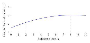
A dose-response curve is a collection of counterfactual means indexed by exposure level.

67.5 Identification Assumptions for Non-Binary Treatments

Causal Assumption

For every \(a\in\mathcal{A}\): \[\text{Consistency:}\qquad A=a\Rightarrow Y=Y(a).\] \[\text{Conditional exchangeability:}\qquad Y(a)\perp\!\!\!\perp A\,\vert\,W.\] \[\text{Positivity:}\qquad f_{A\,\vert\,W}(a\,\vert\,w)>0 \text{ whenever } f_W(w)>0 \text{ and } a \text{ is targeted}.\]

Under these assumptions, \[\begin{aligned} \mathbb{E}\{Y(a)\} &=\mathbb{E}\left[\mathbb{E}\{Y(a)\,\vert\,W\}\right]\\ &=\mathbb{E}\left[\mathbb{E}\{Y(a)\,\vert\,A=a,W\}\right]\\ &=\mathbb{E}\left[\mathbb{E}(Y\,\vert\,A=a,W)\right]. \end{aligned}\] The first equality is the tower rule, the second uses conditional exchangeability, and the third uses consistency.

Identification Result

The dose-response curve is identified by \[\mu(a)=\mathbb{E}\{\mathbb{E}(Y\,\vert\,A=a,W)\}.\] For discrete non-binary \(A\), this formula is evaluated at each exposure category. For continuous \(A\), it is evaluated across exposure values in the target support.

67.6 Positivity With Continuous Treatments

Continuous-treatment positivity is stronger than it first appears. Since \(\mathbb{P}(A=a\,\vert\,W=w)=0\) for any exact point \(a\), positivity is stated in terms of conditional densities. The data must contain enough individuals near exposure level \(a\) for each covariate profile \(w\) being standardized over.

Practical positivity problems arise when:

some exposure values occur only in narrow covariate strata;
the target curve includes doses outside the observed range;
the conditional density \(f_{A\,\vert\,W}(a\,\vert\,w)\) is very small;
scientific interventions at some levels are not meaningful or safe.

Key Idea

For non-binary treatments, the causal estimand is usually a response curve or a contrast along that curve. Identification still uses consistency, exchangeability, and positivity, but positivity becomes a support condition over the exposure distribution.

Lecture 9.2. Multidimensional Exposures

68.1 Radiation Oncology Example

Some exposures are naturally high-dimensional. In radiation oncology, the treatment is not simply “radiation” versus “no radiation.” A patient receives a spatial dose distribution across tissues. For head and neck cancer, dose to salivary glands may affect xerostomia, food intake, and weight loss. Minor changes in where dose is delivered can matter clinically even if the total dose is similar.

Let \(A\) denote a vector of radiation-dose summaries and let \(Y\) denote a secondary outcome such as severe weight loss. A causal question may be: what would the mean outcome be if every patient received dose map \(a\) rather than dose map \(a'\)? \[\mathbb{E}\{Y(a)\}-\mathbb{E}\{Y(a')\}.\] The difficulty is that \(a\) and \(a'\) may be high-dimensional objects rather than simple scalar doses.

68.2 3D Dose Maps

A raw radiation plan can be represented as a three-dimensional voxel map: \[A=(A_1,\ldots,A_p),\] where \(A_j\) is the dose delivered to voxel \(j\). The dimension \(p\) may be very large. The causal response surface \[a\mapsto \mathbb{E}\{Y(a)\}\] is therefore a function over a high-dimensional exposure space.

A spatial exposure such as radiation dose can be encoded as a high-dimensional vector.

68.3 Dose-Volume Summaries

Clinical analyses often replace the full map with lower-dimensional summaries, such as the dose received by each percentile of a gland’s volume. For example, \(A_k\) might be the dose at the \(k\)th percentile, \(k=1,\ldots,100\). This summarizes localization but still leaves a high-dimensional ordered vector.

Such summaries are useful, but they are not automatically causal. If two dose maps have the same summary but different biological effects, the summary loses causally relevant information. If the summary is associated with confounders such as tumor location or disease severity, associational prediction may not recover causal effects.

68.4 High-Dimensional Text Exposures

In natural language processing applications, the exposure may be a document, message, or clinical note. The intervention might alter wording, tone, content, or information ordering. Text can be encoded as word counts, embeddings, topics, or transformer features, but each representation changes the meaning of the intervention.

For causal inference, one must specify what it means to intervene on text. A change in a word embedding is not automatically a meaningful intervention unless it corresponds to an interpretable change in text generation.

68.5 Neuroimaging Exposures

Neuroimaging studies may treat patterns of neural activity, connectivity, or regional activation as exposures. These exposures are structured, correlated, and high-dimensional. A causal claim might concern the effect of activity in a network on behavior, but manipulating one region while holding the rest fixed may be biologically impossible.

68.6 Environmental Mixtures

Environmental epidemiology often studies mixtures: particulate matter, ozone, heavy metals, temperature, humidity, and other exposures occurring jointly. The causal effect of one pollutant may depend on the levels of others, and the positivity condition may fail because some mixtures are never observed.

68.7 Why Multidimensional Treatments Complicate Causal Interpretation

Multidimensional exposures create several linked problems:

Estimand complexity: the response surface \(\mathbb{E}\{Y(a)\}\) is indexed by a high-dimensional \(a\).
Intervention meaning: not every vector \(a\) corresponds to a feasible intervention.
Positivity: the observed data may cover only a small region of the exposure space.
Confounding: high-dimensional exposures are often assigned by complex clinical, environmental, or social processes.
Interpretability: even if a model predicts well, the estimated causal contrast may not map to an actionable intervention.

Key Idea

High-dimensional exposure analysis begins with defining a meaningful intervention. Dimension reduction and machine learning are useful only after the causal estimand is scientifically interpretable.

Lecture 9.3. Causal Dimension Reduction

69.1 Lower-Dimensional Treatment Representations

When \(A\in\mathbb{R}^p\) is high-dimensional, direct estimation of \(a\mapsto\mathbb{E}\{Y(a)\}\) is often infeasible. A natural strategy is to replace \(A\) by a lower-dimensional representation \[G=g(A)\in\mathbb{R}^d,\qquad d<p.\] The goal is not merely to compress \(A\), but to preserve the causal information in \(A\) that is relevant for \(Y\).

69.2 Effect-Preserving Maps \(g(A)\)

Definition 69.1 (Effect-preserving representation). A map \(g:\mathcal{A}\rightarrow\mathcal{G}\) is effect-preserving for the mean counterfactual outcome if \[\mathbb{E}\{Y(a)\}=\theta\{g(a)\}\] for some function \(\theta\) and for all exposure values \(a\) in the target set.

This means that any two exposure values with the same reduced representation have the same mean counterfactual outcome: \[g(a)=g(a')\quad\Rightarrow\quad \mathbb{E}\{Y(a)\}=\mathbb{E}\{Y(a')\}.\] The reduced feature \(g(A)\) is then sufficient for the causal effect of \(A\) on the mean outcome.

69.3 Linear Dimension Reduction \(g(A;\beta)\)

A common model is a linear reduction: \[g(A;\beta)=\beta^\top A,\] or, for \(d>1\), \[g(A;\beta)=\beta^\top A,\qquad \beta\in\mathbb{R}^{p\times d}.\] The causal dimension-reduction condition becomes \[\mathbb{E}\{Y(a)\}=\theta(\beta^\top a).\] Here \(\beta\) defines directions in the exposure space that are causally relevant for the outcome.

Causal dimension reduction seeks a low-dimensional exposure summary that preserves counterfactual means.

69.4 Why PCA Is Insufficient

Principal component analysis finds directions that explain variation in the exposure distribution. It does not use the outcome and does not distinguish causal signal from confounding. A principal component can explain large variation in \(A\) while having no causal effect on \(Y\), and a low-variance component can be highly relevant to \(Y\).

More importantly, preserving the association between \(A\) and \(Y\) is not enough. Because \[\mathbb{E}\{Y(a)\}\ne \mathbb{E}(Y\,\vert\,A=a)\] in the presence of confounding, a dimension-reduction method that optimizes prediction of \(Y\) from \(A\) may preserve confounded associations rather than causal effects.

69.5 Confounding-Aware Dimension Reduction

Under conditional exchangeability, \[\mathbb{E}\{Y(a)\}=\mathbb{E}\{\mathbb{E}(Y\,\vert\,A=a,W)\}.\] A confounding-aware reduction must therefore preserve the standardized outcome regression, not merely the raw conditional mean \(\mathbb{E}(Y\,\vert\,A=a)\). The covariates \(W\) enter because the causal response at \(a\) is obtained by averaging over the target population distribution of \(W\).

One conceptual approach is to search for \(\beta\) such that \[\mathbb{E}\{\mathbb{E}(Y\,\vert\,A=a,W)\} = \theta(\beta^\top a)\] over the exposure values of interest.

69.6 Causal Sufficient Dimension Reduction

Definition 69.2 (Causal sufficient dimension reduction). A reduction \(g(A)\) is causally sufficient for the mean effect of \(A\) if the counterfactual mean depends on \(a\) only through \(g(a)\): \[\mathbb{E}\{Y(a)\}=\mathbb{E}\{Y(a')\} \quad\text{whenever}\quad g(a)=g(a').\]

This definition is about counterfactual distributions, not the observed exposure distribution. Estimating such a reduction requires causal assumptions, adequate support, and a method that accounts for confounding.

Key Idea

Causal dimension reduction is not ordinary compression. It asks for a low-dimensional representation that preserves intervention effects, not just variation in the exposure or prediction of the observed outcome.

Lecture 9.4. Sensitivity Analysis for Unmeasured Confounding

70.1 Violation of Conditional Ignorability

For a binary treatment, the usual identification proof for \(\mathbb{E}\{Y(1)\}\) starts from \[\mathbb{E}\{Y(1)\} = \sum_w\sum_a \mathbb{E}(Y(1)\,\vert\,A=a,W=w)\mathbb{P}(A=a\,\vert\,W=w)\mathbb{P}(W=w).\] Split the sum over \(a\): \[\begin{aligned} \mathbb{E}\{Y(1)\} &= \sum_w \mathbb{E}(Y(1)\,\vert\,A=1,W=w)\mathbb{P}(A=1\,\vert\,W=w)\mathbb{P}(W=w)\\ &\quad+ \sum_w \mathbb{E}(Y(1)\,\vert\,A=0,W=w)\mathbb{P}(A=0\,\vert\,W=w)\mathbb{P}(W=w). \end{aligned}\] The first conditional mean is identified by consistency: \[\mathbb{E}(Y(1)\,\vert\,A=1,W=w)=\mathbb{E}(Y\,\vert\,A=1,W=w).\] The second conditional mean concerns untreated individuals under treatment: \[\mathbb{E}(Y(1)\,\vert\,A=0,W=w).\] It is not observed directly.

If \(Y(1)\perp\!\!\!\perp A\,\vert\,W\), then \[\mathbb{E}(Y(1)\,\vert\,A=0,W=w) = \mathbb{E}(Y(1)\,\vert\,A=1,W=w) = \mathbb{E}(Y\,\vert\,A=1,W=w),\] and the usual adjustment formula follows. If conditional ignorability fails, this replacement is not justified.

70.2 Non-Identifiable Counterfactual Components

The unidentified piece is the distribution of \(Y(1)\) among those with \(A=0\). Similarly, identification of \(\mathbb{E}\{Y(0)\}\) requires information about \(Y(0)\) among those with \(A=1\). These are counterfactual components that the observed data do not reveal without assumptions.

Key Idea

Unmeasured confounding breaks identification because some counterfactual outcome distributions are never observed in the treatment groups where they are needed.

70.3 Bounds Without Sensitivity Parameters

If \(Y\) is bounded, partial identification is possible without specifying a sensitivity model. Suppose \(Y\in[0,1]\). Then \[0\le \mathbb{E}(Y(1)\,\vert\,A=0,W=w)\le 1.\] Therefore \(\mathbb{E}\{Y(1)\}\) is bounded by replacing the unidentified component with 0 or 1: \[\begin{aligned} \sum_w &\mathbb{E}(Y\,\vert\,A=1,W=w)\mathbb{P}(A=1\,\vert\,W=w)\mathbb{P}(W=w)\\ &\le \mathbb{E}\{Y(1)\}\\ &\le \sum_w \left[ \mathbb{E}(Y\,\vert\,A=1,W=w)\mathbb{P}(A=1\,\vert\,W=w) +\mathbb{P}(A=0\,\vert\,W=w) \right]\mathbb{P}(W=w). \end{aligned}\] These bounds are honest but often wide.

70.4 Bounds With Sensitivity Parameters

Sensitivity parameters narrow the set of plausible counterfactual distributions by restricting the magnitude of unmeasured confounding. For example, one might bound the difference \[\left| \mathbb{E}(Y(1)\,\vert\,A=0,W=w)-\mathbb{E}(Y(1)\,\vert\,A=1,W=w) \right| \le \delta.\] For each value of \(\delta\), this yields an interval of possible values for \(\mathbb{E}\{Y(1)\}\) and therefore for the ATE. Reporting the range over plausible \(\delta\) values makes the dependence on untestable assumptions explicit.

70.5 Point Identification With Sensitivity Parameters

Another approach specifies a sensitivity model that maps observed outcome distributions to the unobserved counterfactual distributions. Once the sensitivity parameter is fixed, the causal parameter becomes identified.

70.6 Robins Sensitivity Model

One useful model relates the density of \(Y(1)\) among untreated individuals to the density among treated individuals: \[p(y_1\,\vert\,A=0,W) = \frac{ p(y_1\,\vert\,A=1,W)\exp\{\gamma S(y_1)\} }{ \mathbb{E}[\exp\{\gamma S(Y)\}\,\vert\,A=1,W] }.\] Here \(S(\cdot)\) is a specified function and \(\gamma\) is a sensitivity parameter. When \(\gamma=0\), the two conditional distributions are equal, corresponding to no unmeasured confounding for \(Y(1)\) within strata of \(W\).

Under this model, \[\mathbb{E}(Y(1)\,\vert\,A=0,W=w) = \frac{ \mathbb{E}[Y\exp\{\gamma S(Y)\}\,\vert\,A=1,W=w] }{ \mathbb{E}[\exp\{\gamma S(Y)\}\,\vert\,A=1,W=w] }.\] Thus, for fixed \(\gamma\), \[\begin{aligned} \mathbb{E}\{Y(1)\} &= \sum_w \mathbb{E}(Y\,\vert\,A=1,W=w)\mathbb{P}(A=1\,\vert\,W=w)\mathbb{P}(W=w)\\ &\quad+ \sum_w \frac{ \mathbb{E}[Y\exp\{\gamma S(Y)\}\,\vert\,A=1,W=w] }{ \mathbb{E}[\exp\{\gamma S(Y)\}\,\vert\,A=1,W=w] } \mathbb{P}(A=0\,\vert\,W=w)\mathbb{P}(W=w). \end{aligned}\]

Estimation Notes

A sensitivity analysis workflow is:

Choose a sensitivity model and interpret its parameter scale.
Select a scientifically plausible grid of sensitivity values.
Estimate the identified functional at each value.
Report how the causal conclusion changes across the grid.

Lecture 9.5. Instrumental Variables

71.1 IV Graph

An instrumental variable is a variable \(Z\) that affects treatment \(A\) but is otherwise unrelated to the outcome \(Y\) except through \(A\). It is useful when there is unmeasured confounding between \(A\) and \(Y\).

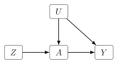
Instrumental variable graph: \(Z\) affects \(Y\) only through \(A\), while \(U\) confounds \(A\) and \(Y\).

71.2 Relevance

Causal Assumption

The instrument must be associated with treatment: \[Z \not\!\perp\!\!\!\perp A.\] In linear models this is often expressed as \[\mathop{\mathrm{Cov}}(Z,A)\ne 0.\]

Relevance is partly empirically checkable because \(Z\) and \(A\) are observed. Weak relevance leads to unstable IV estimates.

71.3 Marginal Ignorability

Causal Assumption

The instrument is marginally independent of the potential outcomes: \[Y(a,z)\perp\!\!\!\perp Z \qquad\text{for all }a,z.\]

This says \(Z\) is as-if randomized with respect to the outcome process. In practice, this is a scientific assumption: an observed association between \(Z\) and baseline covariates may cast doubt on it, but no observed-data test can prove it.

71.4 Exclusion Restriction

Causal Assumption

The instrument has no direct effect on the outcome: \[Y(a,z)=Y(a) \qquad\text{for all }a,z.\]

The exclusion restriction rules out all pathways from \(Z\) to \(Y\) except through \(A\). It is often the most controversial IV assumption.

71.5 Linear Model Assumption

In the simplest linear structural model, suppose variables are standardized and \[A=\gamma_{az}Z+\gamma_{au}U+\epsilon_A,\] \[Y=\gamma_{ya}A+\gamma_{yu}U+\epsilon_Y.\] The causal effect of \(A\) on \(Y\) is \(\gamma_{ya}\). Because \(U\) is unobserved, the ordinary association between \(A\) and \(Y\) is confounded.

71.6 IV Estimand

Under the IV assumptions and the linear model, \[\mathop{\mathrm{Cov}}(Z,Y)=\gamma_{ya}\mathop{\mathrm{Cov}}(Z,A).\] Therefore \[\gamma_{ya}=\frac{\mathop{\mathrm{Cov}}(Z,Y)}{\mathop{\mathrm{Cov}}(Z,A)}.\] If variables are standardized, covariances can be written as correlations: \[\gamma_{ya}=\frac{\operatorname{Corr}(Z,Y)} {\operatorname{Corr}(Z,A)}.\]

71.7 Wald Ratio Intuition

For a binary instrument, the Wald estimand is \[\frac{\mathbb{E}(Y\,\vert\,Z=1)-\mathbb{E}(Y\,\vert\,Z=0)} {\mathbb{E}(A\,\vert\,Z=1)-\mathbb{E}(A\,\vert\,Z=0)}.\] The numerator is the effect of the instrument on the outcome. The denominator is the effect of the instrument on the treatment. If the instrument affects the outcome only by shifting treatment, the ratio rescales the intention-to-treat effect by the amount of treatment movement induced by the instrument. With a binary instrument and a binary or otherwise nonlinear treatment setting, the Wald ratio is commonly interpreted as a LATE or CACE only under additional assumptions such as monotonicity, exclusion, and appropriate independence assumptions; without them, it is not automatically the population ATE.

Identification Result

In a linear IV model with relevance, instrument ignorability, and exclusion, \[\text{causal effect of }A\text{ on }Y = \frac{\mathop{\mathrm{Cov}}(Z,Y)}{\mathop{\mathrm{Cov}}(Z,A)}.\]

71.8 Limitations of IV Analysis

IV analysis is powerful but fragile. Limitations include:

exclusion restrictions are untestable and often scientifically strong;
weak instruments produce unstable estimates;
linear IV identifies a model-specific effect, not necessarily a nonparametric ATE;
with heterogeneous treatment effects, additional assumptions are needed to interpret the estimand as an effect for a particular subpopulation;
invalid instruments can amplify rather than reduce bias.

Key Idea

An instrument replaces adjustment for unmeasured confounding with different untestable assumptions: the instrument must move treatment, be as-if randomized, and affect the outcome only through treatment.

Lecture 9.6. Nonparametric Identification with Unmeasured Variables

72.1 Observed and Unobserved Variables

Let \(V\) denote observed variables and \(U\) denote unobserved variables. A causal graph may be defined over \(V\cup U\), but the analyst only observes the marginal distribution \(p(V)\). The identification question is: \[\mathbb{E}\{Y(a)\}\quad =\quad ?\quad \text{a function of }p(V).\] Nonparametric identification means the answer must hold for every distribution compatible with the graph, without imposing linearity, normality, or other parametric restrictions.

72.2 Adjustment Failure

The adjustment formula works when there is a measured set \(Z\) satisfying the appropriate graphical criterion: \[\mathbb{E}\{Y(a)\}=\mathbb{E}\{\mathbb{E}(Y\,\vert\,A=a,Z)\}.\] If an unmeasured variable lies on an open noncausal path from \(A\) to \(Y\), no observed adjustment set may block the path.

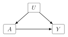
Unmeasured common cause \(U\) creates an open noncausal path between \(A\) and \(Y\).

72.3 Valid Adjustment Sets

If \(U\) is absent, the parents of \(A\) in the causal DAG often provide a valid adjustment set: \[Y(a)\perp\!\!\!\perp A\,\vert\,\mathop{\mathrm{pa}}(A).\] If \(U\) is present but an observed set blocks all noncausal paths, the effect is still identified by adjustment. For example, if \(Z\) blocks the back-door path from \(A\) to \(Y\), then \[\mathbb{E}\{Y(a)\}=\mathbb{E}\{\mathbb{E}(Y\,\vert\,A=a,Z)\}.\]

72.4 Non-Identification

If no valid adjustment set exists, the effect may or may not be identified by some other functional. Non-identification means more than failure of a favorite method. It means there exist two causal models that imply the same observed distribution \(p(V)\) but different values of \(\mathbb{E}\{Y(a)\}\).

Definition 72.1 (Non-identification). A causal parameter \(\psi\) is not identified from \(p(V)\) in a model \(\mathcal{M}\) if there exist two distributions \(P_1,P_2\in\mathcal{M}\) such that \[p_1(V)=p_2(V) \qquad\text{but}\qquad \psi(P_1)\ne \psi(P_2).\]

72.5 Linear SEM Counterexamples

A simple linear structural equation model illustrates the problem. Suppose \[A=\alpha U+\epsilon_A,\] \[Y=\gamma A+\beta U+\epsilon_Y,\] with independent errors. The observed association between \(A\) and \(Y\) can be written schematically as \[\rho_{AY}=\gamma+\alpha\beta.\] The causal effect is \(\gamma\), while \(\alpha\beta\) is the spurious association through the unmeasured common cause. The observed data provide one association but there are two unknown components. Infinitely many pairs \((\gamma,\alpha\beta)\) can produce the same \(\rho_{AY}\).

For example, if \(\rho_{AY}=0.6\), then both of the following are compatible with the same observed association: \[\gamma=0.6,\ \alpha\beta=0, \qquad\text{and}\qquad \gamma=0.1,\ \alpha\beta=0.5.\] The observed distribution alone cannot choose between them.

72.6 Using Submodels to Prove Non-Identification

Non-identification in a simple submodel can be enough to prove non-identification in a larger model. Let \(\mathcal{M}_{\mathrm{sub}}\) be a statistical model contained in a larger model \(\mathcal{M}_{\mathrm{super}}\): \[\mathcal{M}_{\mathrm{sub}}\subset \mathcal{M}_{\mathrm{super}}.\] If a causal parameter is identified in the larger model, then it must also be identified in every smaller submodel: \[\psi \text{ identified in } \mathcal{M}_{\mathrm{super}} \Rightarrow \psi \text{ identified in } \mathcal{M}_{\mathrm{sub}}.\] Taking the contrapositive, \[\psi \text{ not identified in } \mathcal{M}_{\mathrm{sub}} \Rightarrow \psi \text{ not identified in } \mathcal{M}_{\mathrm{super}}.\] This is why a linear structural equation counterexample can prove a nonparametric non-identification result. If even a restricted linear submodel contains two distributions with the same observed law and different causal effects, then the larger nonparametric model also contains those two distributions.

The reverse implication is false. Identification in a linear Gaussian submodel does not imply identification in the unrestricted nonparametric model. A linear model may use algebraic restrictions that are not implied by the graph alone.

72.7 Why Machine Learning Cannot Solve Non-Identification

Machine learning can estimate complex functions of the observed distribution \(p(V)\). It cannot recover information that is not contained in \(p(V)\). If two causal models have the same observed distribution but different causal effects, any algorithm trained only on observed data must return the same output for both models, while the correct causal answers differ.

Key Idea

Non-identification is not a failure of modeling flexibility. It is a logical failure of information: the observed distribution does not contain enough information to determine the causal parameter under the assumed model.

Lecture 9.7. Front-Door Identification

73.1 Front-Door Graph

The front-door model shows that an effect can be identified even when there is unmeasured confounding between treatment and outcome and no valid adjustment set. The key is a measured mediator \(M\) through which all effects of \(A\) on \(Y\) pass.

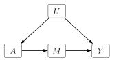
Front-door graph: \(A\) and \(Y\) are confounded by \(U\), but the effect of \(A\) on \(Y\) is fully mediated by observed \(M\).

73.2 Mediator-Based Identification

The graph says that the causal effect decomposes into two parts: \[A\rightarrow M,\qquad M\rightarrow Y.\] The effect of \(A\) on \(M\) is unconfounded. The effect of \(M\) on \(Y\) can be identified by adjusting for \(A\), because the remaining noncausal path from \(M\) to \(Y\) goes through \(A\).

73.3 SWIGs for Front-Door Models

The front-door argument can be expressed with counterfactual independencies: \[M(a)\perp\!\!\!\perp A,\] \[Y(m)\perp\!\!\!\perp M\,\vert\,A,\] \[Y(m)\perp\!\!\!\perp M(a).\] The exclusion-type condition is \[Y(a,m)=Y(m),\] which states that once the mediator is set to \(m\), the value assigned to \(A\) does not further affect \(Y\).

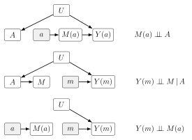
SWIG-style views of the counterfactual independencies used in front-door identification.

73.4 Identification Steps

Start from the distribution of \(Y(a)\): \[p\{Y(a)\}=\sum_m p\{Y(a),M(a)=m\}.\] By the mediation condition, when \(M(a)=m\), \[Y(a)=Y(a,m)=Y(m).\] Thus \[p\{Y(a)\}=\sum_m p\{Y(m),M(a)=m\}.\] Using the counterfactual independence \(Y(m)\perp\!\!\!\perp M(a)\), \[p\{Y(a)\}=\sum_m p\{Y(m)\}p\{M(a)=m\}.\] The mediator distribution is identified because \(M(a)\perp\!\!\!\perp A\) and consistency: \[p\{M(a)=m\}=p(M=m\,\vert\,A=a).\] The remaining term is \[p\{Y(m)\}=\sum_{a'}p\{Y(m)\,\vert\,A=a'\}p(A=a').\] Using \(Y(m)\perp\!\!\!\perp M\,\vert\,A\) and consistency, \[p\{Y(m)\,\vert\,A=a'\}=p(Y\,\vert\,M=m,A=a').\]

73.5 Front-Door Adjustment Formula

Identification Result

For discrete \(A\) and \(M\), the front-door formula is \[\mathbb{E}\{Y(a)\} = \sum_m \left[ \sum_{a'} \mathbb{E}(Y\,\vert\,M=m,A=a')\mathbb{P}(A=a') \right] \mathbb{P}(M=m\,\vert\,A=a).\]

The assigned value \(a\) appears only in the mediator distribution \(\mathbb{P}(M=m\,\vert\,A=a)\). The inner sum identifies the effect of setting the mediator to \(m\) on the outcome by averaging over the treatment distribution.

73.6 Key Assumptions

Causal Assumption

Front-door identification requires:

all directed effects of \(A\) on \(Y\) pass through \(M\);
no unmeasured confounding of \(A\) and \(M\);
no unmeasured confounding of \(M\) and \(Y\) after conditioning on \(A\);
positivity for the relevant treatment and mediator levels.

If there is a direct arrow \(A\rightarrow Y\), then \(Y(a,m)=Y(m)\) fails. If there is unmeasured confounding between \(A\) and \(M\), then \(p(M(a))\) is not identified from \(p(M\,\vert\,A=a)\). If there is unmeasured confounding between \(M\) and \(Y\) within levels of \(A\), then the mediator effect is not identified.

73.7 Practical Implications

The front-door formula is rarely justified automatically. It requires a mediator that captures the entire causal effect of treatment and is itself sufficiently well measured. Nevertheless, it is important because it proves that adjustment is not the only route to nonparametric identification.

73.8 Extensions and Software

Modern identification algorithms generalize front-door reasoning to larger graphs with hidden variables. Software can take a graph with observed and hidden variables and return an identifying functional when one exists. Estimation then requires fitting the conditional distributions appearing in that functional, often with one-step or TMLE-style estimators.

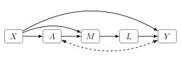
Extended front-door-type graphs can be identifiable even when no ordinary adjustment set exists.

Implementation Notes

Graph-based software for hidden-variable causal models typically asks the user to provide the observed variables, directed edges, hidden-variable or bidirected edges, the treatment, and the outcome. The software then checks whether the effect is identifiable and, when possible, returns an identifying functional and estimators such as one-step or TMLE estimators. The graph specification is part of the statistical analysis; changing the graph changes the estimand that can be identified.

Key Idea

Front-door identification works by replacing an unidentifiable direct treatment effect with two identifiable pieces: the effect of treatment on mediator and the effect of mediator on outcome.

Lecture 9.8. Missing Data: Traditional Statistical View

74.1 Target Estimands With Incomplete Data

Missing data problems begin with a target estimand defined for a complete-data distribution. Examples include \[\psi_1=\mathbb{E}(Y),\] \[\psi_2=\mathbb{E}(Y\,\vert\,X=x),\] and, under causal assumptions, \[\psi_3=\mathbb{E}\{\mathbb{E}(Y\,\vert\,X,T=1)-\mathbb{E}(Y\,\vert\,X,T=0)\}.\] These estimands are functions of variables such as \((X,T,Y)\) that may not be fully observed for every sampled unit.

74.2 Missingness Indicators

Let \(V\) be a variable that may be missing. Define \[R_V= \begin{cases} 1, & V \text{ is observed},\\ 0, & V \text{ is missing}. \end{cases}\] The observed version is \[V^*= \begin{cases} V, & R_V=1,\\ ?, & R_V=0. \end{cases}\] If \(X,T,Y\) can all be missing, then the observed data include \[X^*,T^*,Y^*,R_X,R_T,R_Y.\]

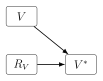
The observed variable \(V^*\) is determined by the full value \(V\) and the missingness indicator \(R_V\).

74.3 Complete-Case Analysis

Complete-case analysis discards any row with missing values in variables needed for the analysis. It is simple, but it changes the target population from all sampled units to units with complete records. It is unbiased for some estimands only under strong missingness conditions, such as missingness independent of the variables relevant to the estimand.

74.4 Imputation

Imputation replaces missing values with predicted or sampled values. Single imputation fills in one value; multiple imputation creates several completed data sets and combines results. Imputation can improve efficiency relative to complete-case analysis, but it depends on assumptions about the missingness mechanism and the imputation model.

Imputation should not be viewed as a purely technical repair. It encodes assumptions about what the missing values would have been.

74.5 Efficiency Loss

Ignoring incomplete rows reduces sample size and can discard partially observed information. For example, a row with \(X\) and \(T\) observed but \(Y\) missing still contains information about the distribution of covariates and treatment. A row with \(Y\) observed but one covariate missing still contains outcome information. Efficient methods use all observed components compatible with the identifying assumptions.

74.6 Bias From Missingness

Bias occurs when complete cases differ systematically from incomplete cases in ways related to the target estimand. For example, if people with severe disease are less likely to report an outcome, the observed outcome mean among respondents can underestimate the true mean. If missingness depends on the unobserved value itself, naive analyses can be badly biased.

74.7 Sources of Missing Data

Common sources include:

random data-entry failures;
survey nonresponse to sensitive questions;
variables introduced partway through a study;
measurement limits, such as values too fast or too small to record;
dropout or loss to follow-up;
clinician decisions about whether to order a test.

Different sources imply different assumptions. A randomly skipped data-entry field is not the same as a refused sensitive survey question or a diagnostic test ordered only for high-risk patients.

Key Idea

Missing data analysis is an identification problem. Before choosing complete cases, imputation, or weighting, specify the target complete-data estimand and the assumptions linking observed records to missing values.

Lecture 9.9. Rubin’s Missingness Hierarchy

75.1 Missing Completely at Random

Definition 75.1 (Missing completely at random). Missingness is missing completely at random (MCAR) if the probability of missingness does not depend on any data values, observed or unobserved. \[R\perp\!\!\!\perp(X_{\mathrm{obs}},X_{\mathrm{mis}},Z), \qquad p(R\,\vert\,X,Z)=p(R).\]

MCAR is like randomly removing entries from a data set. Complete cases are a random subsample with respect to the variables in the full data. This is a strong condition and often implausible in medical and social data.

75.2 Missing at Random

Definition 75.2 (Missing at random). Missingness is missing at random (MAR) if the probability of missingness may depend on observed information but not on missing values after conditioning on the observed information: \[R\perp\!\!\!\perp X_{\mathrm{mis}}\,\vert\,Z,X_{\mathrm{obs}}, \qquad p(R\,\vert\,X,Z)=p(R\,\vert\,Z,X_{\mathrm{obs}}).\]

For example, outcome missingness may depend on age and sex if those variables are observed for everyone. Under MAR, methods such as inverse probability weighting and multiple imputation can be justified if the models are correctly specified.

75.3 Missing Not at Random

Definition 75.3 (Missing not at random). Missingness is missing not at random (MNAR) if the probability of missingness depends on missing values themselves, even after conditioning on observed information.

For example, income may be missing because high-income respondents choose not to report it, or substance-use history may be missing because people with substance-use history refuse to answer. MNAR is not one model; it is a broad category containing many different mechanisms.

75.4 Statistical Definitions Using \(R\), \(X_{\text{obs}}\), \(X_{\text{miss}}\), and \(Z\)

Let \(Z\) denote variables observed for all units. Let \(X\) denote variables subject to missingness, decomposed into observed and missing parts: \[X=(X_{\mathrm{obs}},X_{\mathrm{mis}}).\] Let \(R\) denote the missingness pattern. The hierarchy can be summarized as: \[\text{MCAR:}\qquad p(R\,\vert\,X,Z)=p(R),\] \[\text{MAR:}\qquad p(R\,\vert\,X,Z)=p(R\,\vert\,X_{\mathrm{obs}},Z),\] \[\text{MNAR:}\qquad p(R\,\vert\,X,Z) \text{ depends on }X_{\mathrm{mis}}\text{ for at least one pattern}.\]

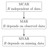
Rubin’s hierarchy classifies missingness by what information predicts missingness.

75.5 Limitations of MCAR/MAR/MNAR

The hierarchy is useful but incomplete. Its limitations include:

MCAR and MAR are statistical restrictions, not causal explanations.
MNAR is too broad: many distinct mechanisms are all labeled MNAR.
The hierarchy can be hard to apply when several variables are missing.
It does not automatically tell us whether a target estimand is recoverable.
It does not by itself specify an estimation strategy.

Key Idea

MCAR, MAR, and MNAR describe how missingness probabilities relate to observed and unobserved values. They are useful labels, but causal graphs provide a more explicit language for why values are missing and what can be recovered.

Lecture 9.10. Causal and Counterfactual Views of Missing Data

76.1 Why Missingness Is Causal

Missingness can be viewed as a causal process. Let \(R_k\) indicate whether variable \(L_k\) is observed. Intervening to set \(R_k=1\) corresponds to forcing the variable to be measured. The full value can be written as a counterfactual quantity: \[L_k(1)=\text{the value of }L_k\text{ that would be recorded if }R_k=1.\] The factual observed value is \[L_k= \begin{cases} L_k(1), & R_k=1,\\ ?, & R_k=0. \end{cases}\] Thus missing data involve counterfactuals: values that would have been observed under a measurement intervention.

76.2 Missing Data DAGs

A missing data DAG contains full-data variables, missingness indicators, and observed coarsened variables. For one partially observed variable:

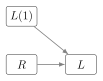
Basic missing-data structure: the observed value is determined by the full value and its missingness indicator.

With several variables, missingness indicators may depend on full values, observed values, other indicators, or completely observed covariates \(Z\). Graphical restrictions encode assumptions about these dependencies.

76.3 Full-Law Factorization

Let \(Z\) denote completely observed variables, \(L(1)\) the full-data variables that would be observed under measurement, \(R\) the missingness indicators, and \(L\) the coarsened observed variables. The full law can be factored as \[p\{Z,L(1),R,L\} = p\{Z,L(1)\}\, p\{R\,\vert\,L(1),Z\}\, p\{L\,\vert\,L(1),R,Z\}.\] The first factor is the target full-data law. The second factor is the missingness mechanism. The third factor is deterministic once the consistency rule is specified: \[L_k= \begin{cases} L_k(1), & R_k=1,\\ ?, & R_k=0. \end{cases}\] The observed-data law is obtained after marginalizing over the unobserved components of \(L(1)\).

76.4 Recoverability

Definition 76.1 (Recoverability). A target full-data parameter is recoverable if it can be written as a function of the observed-data distribution.

Recoverability is the missing-data analogue of causal identification. For example, the full-data mean \(\mathbb{E}\{L(1)\}\) is recoverable under suitable missingness assumptions, but may not be recoverable if missingness depends on the unobserved value in an unrestricted way.

76.5 Missingness Mechanisms as Graphs

Consider two partially observed variables, smoking status \(L_1(1)\) and bronchitis status \(L_2(1)\), with indicators \(R_1\) and \(R_2\). Different arrows tell different stories:

\(L_2(1)\rightarrow R_1\): inquiry about smoking depends on true bronchitis status.
\(R_1\rightarrow R_2\): whether a diagnostic test is ordered depends on whether smoking was assessed.
\(L_1\rightarrow R_2\): observed smoking status affects diagnostic testing.
\(L_1(1)\rightarrow R_2\): true smoking status affects diagnostic testing, even when smoking status is not observed.

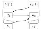
A missing-data DAG can encode how true values, observed values, and measurement decisions interact.

76.6 Graphical MCAR, MAR, and MNAR

Graphically:

MCAR means there are no arrows into missingness indicators from data variables or other missingness-relevant variables.
MAR means missingness indicators may depend on completely observed variables and observed values, but not on full values that are hidden when missing.
MNAR means at least one missingness indicator has a parent among the full-data variables whose values may be unobserved.

The graph is more informative than a label because it records which variables drive which missingness decisions.

76.7 Workflow for Missing Data Analysis

Estimation Notes

A graphical missing-data workflow is:

Define the full-data estimand, such as \(\mathbb{E}\{L(1)\}\) or a causal effect.
Draw a graph over full-data variables, missingness indicators, observed coarsened variables, and completely observed variables.
Assess recoverability: can the estimand be written using the observed data law?
If recoverable, estimate the identifying functional with regression, weighting, imputation, TMLE, or another appropriate method.
If not recoverable, report bounds, perform sensitivity analysis, or collect additional data.

76.8 Connections to Censoring Bias

Censoring is a special case of missingness over time. In survival analysis, a future outcome is missing after dropout. Treating censoring indicators as time-varying treatment variables leads to the same identification logic used for longitudinal interventions: consistency, exchangeability for the censoring process, and positivity of remaining uncensored.

Key Idea

The causal view treats missingness indicators as intervention variables and missing values as counterfactual full-data quantities. This turns missing-data analysis into a recoverability problem, parallel to causal identification.

Chapter 1. Review of Key Statistical Concepts

Lecture 1.1. Populations, Parameters, Estimators, and Inference

1.1 Target Population

1.2 Target Parameter and Estimand

1.3 Data as a Sample from a Population

1.4 Point Estimates and Estimators

1.5 Standard Errors

1.6 Confidence Intervals

1.7 Hypothesis Tests

Lecture 1.2. Frequentist and Bayesian Perspectives

2.1 Frequentist Interpretation of Probability

2.2 Bayesian Updating

2.3 Repeated-Sampling Properties

2.4 Bias

2.5 Sampling Distribution

2.6 Coverage Probability

2.7 Power

Lecture 1.3. Probability Foundations

3.1 Joint Distributions

3.2 Marginal Distributions

3.3 Conditional Distributions

3.4 Chain Rule Factorization

3.5 Bayes Rule

3.6 From Joint to Marginal Probabilities

3.7 Conditional Probability as Subgroup Proportion

Lecture 1.4. Independence and Conditional Independence

4.1 Definition of Independence

4.2 Definition of Conditional Independence

4.3 Independence in Randomized Trials

4.4 Stratified Randomization

4.5 Why Conditioning Can Remove Information

4.6 Why Conditional Independence Matters for Causal Inference

Lecture 1.5. Expectation and Conditional Expectation

5.1 Expected Value

5.2 Expectation of Transformations

5.3 Binary Variables and Probabilities

5.4 Conditional Expectation as Subgroup Mean

5.5 Conditional Mean as a Function

5.6 Interpreting \(\mathbb{E}(Y\,\vert\,A,W)\)

Lecture 1.6. The Tower Rule

6.1 Plain-Language Statement of the Tower Rule

6.2 Weighted Averages of Subgroup Means

6.3 Numeric Example

6.4 Probability Notation

6.5 Shorthand Form: \(\mathbb{E}(W)=\mathbb{E}\{\mathbb{E}(W\,\vert\,A)\}\)

6.6 Common Mistakes

6.7 Proof of the Tower Rule

6.8 Practice Problems

Lecture 1.7. Regression as Conditional Expectation Estimation

7.1 Regression as Estimation of \(\mathbb{E}(Y\,\vert\,A,W)\)

7.2 Linear Regression

7.3 Logistic Regression

7.4 Generalized Linear Models

7.5 Main-Terms Models

7.6 Interaction Models

7.7 Using glm in R

7.8 Prediction with newdata

7.9 Regression Output as Subgroup Mean Estimates

Pooling.

Stratifying.

Chapter 2. Asking Causal Questions

Lecture 2.1. From Association to Causation

8.1 Motivating Example: Early Imaging for Back Pain

8.2 Associative Analysis

8.3 Causal Analysis

8.4 Population under Intervention

8.5 Why Data Alone Cannot Answer Causal Questions

8.6 Untestable Assumptions

Lecture 2.2. The Roadmap for Causal Analysis

9.1 Overview

9.2 Specify a Causal Model

9.3 Specify a Causal Question and Parameter

9.4 Link Observed Data to the Causal Model

9.5 Assess Identifiability

9.6 Specify Statistical Parameter and Model

9.7 Estimate

9.8 Interpret

Lecture 2.3. Causal Models and DAGs

10.1 Why Graphical Models

10.2 Directed Acyclic Graphs

7.7 Using `glm` in R

7.8 Prediction with `newdata`