← Study Notes

Computing and AI

Machine Learning

English · 194 pp. PDF

Open PDF ↗ Download PDF ↓

Contents

1. Part 0: Introduction & Mathematical Foundations
2. 1 What is Machine Learning?
   1. 1.1 Core Definitions and Philosophy
   2. 1.2 Types of Machine Learning
   3. 1.3 Machine Learning vs AI vs Statistics
   4. 1.4 Major Paradigms and Milestones
3. 2 Mathematical Foundations
   1. 2.1 Linear Algebra Refresher
   2. 2.2 Probability Theory
   3. 2.3 Calculus for Machine Learning
   4. 2.4 Optimization Basics
   5. 2.5 Summary of Part 0
4. Part 1: Supervised Learning (Classical Models)
5. 3 Regression Models
   1. 3.1 Linear Regression
   2. 3.2 Regularization
   3. 3.3 Polynomial Regression and Basis Expansion
   4. 3.4 Logistic Regression
6. 4 Distance-Based Models
   1. 4.1 K-Nearest Neighbors (KNN)
   2. 4.2 Distance Metrics
   3. 4.3 Weighted KNN
   4. 4.4 The Curse of Dimensionality
   5. 4.5 Choosing k
7. 5 Decision Trees and Rule-Based Methods
   1. 5.1 Decision Tree Basics
   2. 5.2 Splitting Criteria
   3. 5.3 Tree Growing Algorithms
   4. 5.4 Regression Trees
   5. 5.5 Pruning
   6. 5.6 Interpretability vs Performance
8. 6 Bias–Variance Tradeoff
   1. 6.1 Decomposition of Prediction Error
   2. 6.2 Understanding Bias and Variance
   3. 6.3 Model Complexity and the Tradeoff
   4. 6.4 Examples by Model Type
   5. 6.5 Controlling the Tradeoff
   6. 6.6 Summary of Part 1
9. Part 2: Probabilistic Models
10. 7 Naive Bayes
    1. 7.1 Probabilistic Classification Framework
    2. 7.2 The Naive Bayes Assumption
    3. 7.3 Estimating Parameters
    4. 7.4 Variants of Naive Bayes
    5. 7.5 Applications
11. 8 Generative vs Discriminative Models
    1. 8.1 Key Distinction
    2. 8.2 Gaussian Discriminant Analysis (GDA)
    3. 8.3 Hidden Markov Models (Brief Overview)
12. 9 Support Vector Machines
    1. 9.1 Intuition: Maximum Margin Classification
    2. 9.2 Mathematical Formulation (Hard Margin)
    3. 9.3 Lagrange Duality and the Dual Form
    4. 9.4 The Kernel Trick
    5. 9.5 Soft Margin SVM
    6. 9.6 Support Vector Regression (SVR)
    7. 9.7 Practical Considerations
    8. 9.8 Summary of Part 2
13. Part 3: Ensemble Methods
14. 10 Introduction to Ensemble Learning
15. 11 Bagging (Bootstrap Aggregating)
    1. 11.1 Bootstrap Sampling
    2. 11.2 Bagging Algorithm
    3. 11.3 Random Forests
    4. 11.4 Out-of-Bag (OOB) Error Estimation
    5. 11.5 Feature Importance in Random Forests
    6. 11.6 Advantages and Limitations
16. 12 Boosting
    1. 12.1 Boosting Philosophy
    2. 12.2 AdaBoost (Adaptive Boosting)
    3. 12.3 Gradient Boosting
    4. 12.4 XGBoost (Extreme Gradient Boosting)
    5. 12.5 LightGBM and CatBoost
    6. 12.6 Regularization in Boosting
    7. 12.7 When to Use Boosting vs Bagging
17. 13 Stacking and Blending
    1. 13.1 Stacking (Stacked Generalization)
    2. 13.2 Blending
    3. 13.3 Choosing Base Models
    4. 13.4 Practical Implementation
    5. 13.5 Multi-Level Stacking
    6. 13.6 Summary of Part 3
18. Part 4: Neural Networks and Deep Learning
19. 14 The Perceptron
    1. 14.1 The Perceptron Model
    2. 14.2 Perceptron Learning Algorithm
    3. 14.3 Limitations of the Perceptron
20. 15 Artificial Neural Networks
    1. 15.1 The Neuron Model
    2. 15.2 Activation Functions
    3. 15.3 Multi-Layer Perceptron (MLP)
    4. 15.4 Forward Propagation
    5. 15.5 Loss Functions
    6. 15.6 Backpropagation
    7. 15.7 Vanishing and Exploding Gradients
21. 16 Optimization in Deep Learning
    1. 16.1 Stochastic Gradient Descent Variants
    2. 16.2 Learning Rate Schedules
    3. 16.3 Batch Normalization
    4. 16.4 Dropout
22. 17 Deep Architectures
    1. 17.1 Convolutional Neural Networks (CNNs)
    2. 17.2 Recurrent Neural Networks (RNNs)
    3. 17.3 Transformers and Attention
    4. 17.4 Summary of Part 4
23. Part 5: Unsupervised Learning
24. 18 Introduction to Unsupervised Learning
25. 19 Clustering
    1. 19.1 K-Means Clustering
    2. 19.2 Hierarchical Clustering
    3. 19.3 DBSCAN (Density-Based Clustering)
    4. 19.4 Cluster Evaluation Metrics
26. 20 Dimensionality Reduction
    1. 20.1 Motivation
    2. 20.2 Principal Component Analysis (PCA)
    3. 20.3 Linear Discriminant Analysis (LDA)
    4. 20.4 Non-Linear Methods
27. 21 Association Rule Learning
    1. 21.1 Market Basket Analysis
    2. 21.2 Apriori Algorithm
    3. 21.3 Applications
    4. 21.4 Summary of Part 5
28. Part 6: Model Evaluation & Practical Aspects
29. 22 Model Evaluation Metrics
    1. 22.1 Classification Metrics
    2. 22.2 Regression Metrics
30. 23 Model Selection and Hyperparameter Tuning
    1. 23.1 Cross-Validation
    2. 23.2 Hyperparameter Tuning
    3. 23.3 Nested Cross-Validation
31. 24 Data Preprocessing
    1. 24.1 Feature Scaling
    2. 24.2 Encoding Categorical Variables
    3. 24.3 Handling Missing Data
    4. 24.4 Outlier Detection and Treatment
32. 25 Feature Engineering
    1. 25.1 Feature Extraction vs Selection
    2. 25.2 Feature Selection Methods
    3. 25.3 Domain-Specific Feature Engineering
    4. 25.4 Summary of Part 6
33. Part 7: Tools, Pipelines, and Deployment
34. 26 WEKA: Practical Guide
    1. 26.1 Introduction to WEKA
    2. 26.2 WEKA Explorer Interface
    3. 26.3 Data Format: ARFF
    4. 26.4 Workflow Example: Classification
    5. 26.5 Common WEKA Algorithms
    6. 26.6 Visualizing Results
    7. 26.7 Advantages and Limitations
35. 27 ML Pipelines in Python
    1. 27.1 Introduction to Scikit-learn
    2. 27.2 The Pipeline Concept
    3. 27.3 Building Pipelines
    4. 27.4 Column Transformer
    5. 27.5 Pipeline with GridSearchCV
    6. 27.6 Custom Transformers
    7. 27.7 Model Persistence
    8. 27.8 Complete Pipeline Example
36. 28 Model Deployment
    1. 28.1 Deployment Considerations
    2. 28.2 Model Export Formats
    3. 28.3 Serving Models via REST API
    4. 28.4 Containerization with Docker
    5. 28.5 Cloud Deployment
    6. 28.6 Model Monitoring
    7. 28.7 Best Practices Summary
    8. 28.8 Summary of Part 7
37. Part 8: Advanced Topics and Modern Directions
38. 29 Reinforcement Learning
    1. 29.1 Introduction to Reinforcement Learning
    2. 29.2 Core Components
    3. 29.3 The Exploration-Exploitation Dilemma
    4. 29.4 Q-Learning
    5. 29.5 Deep Q-Networks (DQN)
    6. 29.6 Policy Gradient Methods
    7. 29.7 Applications of RL
39. 30 Representation Learning
    1. 30.1 Introduction to Representation Learning
    2. 30.2 Autoencoders
    3. 30.3 Word Embeddings
    4. 30.4 Contrastive Learning
40. 31 Ethics and Fairness in Machine Learning
    1. 31.1 Bias and Discrimination
    2. 31.2 Fairness Definitions
    3. 31.3 Explainable AI (XAI)
    4. 31.4 Responsible AI Practices
41. 32 Modern Trends
    1. 32.1 Transfer Learning and Fine-Tuning
    2. 32.2 Foundation Models
    3. 32.3 Federated Learning
    4. 32.4 AutoML (Automated Machine Learning)
    5. 32.5 Future Directions
    6. 32.6 Conclusion

Part 0: Introduction & Mathematical Foundations

1 What is Machine Learning?

1.1 Core Definitions and Philosophy

Definition 1.1 (Machine Learning). Machine Learning is a field of study that gives computers the ability to learn from data without being explicitly programmed. More formally, a program is said to learn from experience \(E\) with respect to some task \(T\) and performance measure \(P\), if its performance on \(T\), as measured by \(P\), improves with experience \(E\).

Intuition 2. Think of teaching a child to recognize cats. Instead of writing down explicit rules (“has whiskers, four legs, pointy ears”), you show them many pictures of cats and non-cats. Over time, they learn the pattern themselves. Machine learning works similarly—we provide data (experience), and the algorithm discovers the patterns.

Example 1.3 (Email Spam Filter).

• Task \(T\): Classify emails as spam or not spam

• Experience \(E\): A dataset of emails labeled as spam/not spam

• Performance \(P\): Accuracy of classification on new emails

The algorithm learns from labeled examples and improves its classification accuracy over time.

1.2 Types of Machine Learning

Machine learning paradigms are categorized by the type of feedback available during training:

1.2.1 Supervised Learning

In supervised learning, we have a dataset \(\mathcal{D} = \{(\boldsymbol{x}_1, y_1), (\boldsymbol{x}_2, y_2), \ldots, (\boldsymbol{x}_n, y_n)\}\) where \(\boldsymbol{x}_i \in \mathbb{R}^d\) are input features and \(y_i\) are labels.

• Classification: \(y_i\) is categorical (e.g., spam/not spam, cat/dog/bird)

• Regression: \(y_i\) is continuous (e.g., house prices, temperature)

Goal: Learn a function \(f: \mathbb{R}^d \to \mathcal{Y}\) such that \(f(\boldsymbol{x}) \approx y\) for new, unseen examples.

Example 1.4 (Supervised Learning Applications).

• Predicting house prices from size, location, number of rooms (regression)

• Diagnosing diseases from medical images (classification)

• Speech recognition (classification)

1.2.2 Unsupervised Learning

In unsupervised learning, we only have inputs \(\mathcal{D} = \{\boldsymbol{x}_1, \boldsymbol{x}_2, \ldots, \boldsymbol{x}_n\}\) without labels.

Goal: Discover hidden structure or patterns in the data.

• Clustering: Group similar examples together

• Dimensionality Reduction: Find lower-dimensional representations

• Density Estimation: Model the probability distribution of data

Example 1.5 (Unsupervised Learning Applications).

• Customer segmentation in marketing

• Anomaly detection in network traffic

• Topic modeling in document collections

1.2.3 Semi-Supervised Learning

A middle ground where we have a small amount of labeled data and a large amount of unlabeled data. This is common in practice since labeling is expensive.

1.2.4 Reinforcement Learning

An agent learns to make decisions by interacting with an environment, receiving rewards or penalties for actions.

• Agent: The learner/decision maker

• Environment: What the agent interacts with

• Actions: Choices available to the agent

• Rewards: Feedback signal (positive or negative)

Example 1.6 (Reinforcement Learning). Teaching a robot to walk: it tries different leg movements (actions), and receives positive reward when it moves forward and negative reward when it falls.

1.3 Machine Learning vs AI vs Statistics

Key Idea

Artificial Intelligence (AI): The broad goal of creating intelligent machines. ML is a subset of AI.

Machine Learning (ML): Algorithms that improve through experience. Focus on prediction and pattern recognition.

Statistics: The science of collecting, analyzing, and interpreting data. ML borrows heavily from statistics but emphasizes prediction over inference.

The line between ML and statistics is blurry. Roughly: statistics asks “What can we infer?” while ML asks “What can we predict?”

1.4 Major Paradigms and Milestones

• 1950s-60s: Perceptron, early neural networks

• 1980s: Backpropagation algorithm

• 1990s: Support Vector Machines, Random Forests

• 2000s: Deep learning resurgence, big data

• 2010s: AlexNet (2012), AlphaGo (2016), Transformers (2017)

• 2020s: Large language models (GPT, BERT), foundation models

2 Mathematical Foundations

2.1 Linear Algebra Refresher

2.1.1 Vectors and Vector Spaces

Definition 2.1 (Vector). A vector \(\boldsymbol{v} \in \mathbb{R}^n\) is an ordered list of \(n\) real numbers: \[\boldsymbol{v} = \begin{bmatrix} v_1 \\ v_2 \\ \vdots \\ v_n \end{bmatrix}\] We denote vectors in bold lowercase (e.g., \(\boldsymbol{x}, \boldsymbol{w}\)).

Geometric Interpretation: A vector represents a point in \(n\)-dimensional space or a direction with magnitude.

Definition 2.2 (Vector Operations). For \(\boldsymbol{u}, \boldsymbol{v} \in \mathbb{R}^n\) and scalar \(\alpha \in \mathbb{R}\):

• Addition: \(\boldsymbol{u} + \boldsymbol{v} = [u_1+v_1, u_2+v_2, \ldots, u_n+v_n]^\top\)

• Scalar multiplication: \(\alpha \boldsymbol{v} = [\alpha v_1, \alpha v_2, \ldots, \alpha v_n]^\top\)

• Dot product: \(\boldsymbol{u} \cdot \boldsymbol{v} = \boldsymbol{u}^\top \boldsymbol{v} = \sum_{i=1}^n u_i v_i\)

Intuition 9. The dot product \(\boldsymbol{u} \cdot \boldsymbol{v}\) measures how much two vectors point in the same direction: \[\boldsymbol{u} \cdot \boldsymbol{v} = \left\lVert\boldsymbol{u}\right\rVert \left\lVert\boldsymbol{v}\right\rVert \cos\theta\] where \(\theta\) is the angle between them. If \(\theta = 90^{\circ}\), then \(\boldsymbol{u} \cdot \boldsymbol{v} = 0\) (orthogonal).

Definition 2.4 (Norm). The Euclidean norm (or \(\ell_2\)-norm) of a vector \(\boldsymbol{v}\) is: \[\left\lVert\boldsymbol{v}\right\rVert_2 = \sqrt{\sum_{i=1}^n v_i^2} = \sqrt{\boldsymbol{v}^\top \boldsymbol{v}}\] Other common norms include \(\ell_1\)-norm: \(\left\lVert\boldsymbol{v}\right\rVert_1 = \sum_{i=1}^n |v_i|\) and \(\ell_\infty\)-norm: \(\left\lVert\boldsymbol{v}\right\rVert_\infty = \max_i |v_i|\).

2.1.2 Matrices

Definition 2.5 (Matrix). A matrix \(\boldsymbol{A} \in \mathbb{R}^{m \times n}\) is a rectangular array with \(m\) rows and \(n\) columns: \[\boldsymbol{A} = \begin{bmatrix} a_{11} & a_{12} & \cdots & a_{1n} \\ a_{21} & a_{22} & \cdots & a_{2n} \\ \vdots & \vdots & \ddots & \vdots \\ a_{m1} & a_{m2} & \cdots & a_{mn} \end{bmatrix}\] We denote matrices in bold uppercase (e.g., \(\boldsymbol{X}, \boldsymbol{W}\)).

Definition 2.6 (Matrix-Vector Multiplication). For \(\boldsymbol{A} \in \mathbb{R}^{m \times n}\) and \(\boldsymbol{x} \in \mathbb{R}^n\): \[\boldsymbol{A}\boldsymbol{x} = \begin{bmatrix} \boldsymbol{a}_1^\top \boldsymbol{x} \\ \boldsymbol{a}_2^\top \boldsymbol{x} \\ \vdots \\ \boldsymbol{a}_m^\top \boldsymbol{x} \end{bmatrix} \in \mathbb{R}^m\] where \(\boldsymbol{a}_i^\top\) is the \(i\)-th row of \(\boldsymbol{A}\).

Key Point: Matrix multiplication \(\boldsymbol{A}\boldsymbol{x}\) is a linear transformation that maps \(\boldsymbol{x}\) to a new vector.

Definition 2.7 (Matrix-Matrix Multiplication). For \(\boldsymbol{A} \in \mathbb{R}^{m \times n}\) and \(\boldsymbol{B} \in \mathbb{R}^{n \times p}\): \[(\boldsymbol{A}\boldsymbol{B})_{ij} = \sum_{k=1}^n a_{ik} b_{kj}\] Result is \(\boldsymbol{C} \in \mathbb{R}^{m \times p}\).

Definition 2.8 (Transpose). The transpose of \(\boldsymbol{A} \in \mathbb{R}^{m \times n}\) is \(\boldsymbol{A}^\top \in \mathbb{R}^{n \times m}\) where \((\boldsymbol{A}^\top)_{ij} = a_{ji}\).

A matrix is symmetric if \(\boldsymbol{A} = \boldsymbol{A}^\top\).

Definition 2.9 (Identity and Inverse). The identity matrix \(\boldsymbol{I}_n \in \mathbb{R}^{n \times n}\) has 1s on the diagonal and 0s elsewhere: \(\boldsymbol{I}_n \boldsymbol{x} = \boldsymbol{x}\) for all \(\boldsymbol{x}\).

The inverse of a square matrix \(\boldsymbol{A}\) (if it exists) is \(\boldsymbol{A}^{-1}\) such that \(\boldsymbol{A}\boldsymbol{A}^{-1} = \boldsymbol{A}^{-1}\boldsymbol{A} = \boldsymbol{I}\).

2.1.3 Eigenvalues and Eigenvectors

Definition 2.10 (Eigenvalue and Eigenvector). For a square matrix \(\boldsymbol{A} \in \mathbb{R}^{n \times n}\), a non-zero vector \(\boldsymbol{v}\) is an eigenvector with eigenvalue \(\lambda\) if: \[\boldsymbol{A}\boldsymbol{v} = \lambda \boldsymbol{v}\] This means \(\boldsymbol{A}\) stretches \(\boldsymbol{v}\) by factor \(\lambda\) without changing its direction.

Intuition 17. Eigenvectors are special directions that are only scaled (not rotated) by the matrix transformation. They reveal the “natural axes” of the transformation.

Definition 2.12 (Eigendecomposition). A symmetric matrix \(\boldsymbol{A} \in \mathbb{R}^{n \times n}\) can be decomposed as: \[\boldsymbol{A} = \boldsymbol{Q}\boldsymbol{\Lambda}\boldsymbol{Q}^\top\] where \(\boldsymbol{Q}\) contains orthonormal eigenvectors as columns, and \(\boldsymbol{\Lambda}\) is diagonal with eigenvalues.

Importance in ML: Eigendecomposition is crucial for PCA, understanding optimization landscapes, and analyzing neural network behavior.

2.2 Probability Theory

2.2.1 Random Variables and Distributions

Definition 2.13 (Random Variable). A random variable \(X\) is a function that maps outcomes of a random experiment to real numbers. It can be:

• Discrete: Takes countable values (e.g., dice roll, coin flip)

• Continuous: Takes values in an interval (e.g., height, temperature)

Definition 2.14 (Probability Mass Function (PMF)). For discrete \(X\), the PMF is \(P(X = x)\), satisfying: \[P(X = x) \geq 0, \quad \sum_x P(X = x) = 1\]

Definition 2.15 (Probability Density Function (PDF)). For continuous \(X\), the PDF \(p(x)\) satisfies: \[p(x) \geq 0, \quad \int_{-\infty}^\infty p(x)\,dx = 1, \quad P(a \leq X \leq b) = \int_a^b p(x)\,dx\]

Example 2.16 (Important Distributions).

• Bernoulli: \(X \in \{0,1\}\), \(P(X=1) = p\). Models binary outcomes (coin flip).

• Gaussian (Normal): \(X \sim \mathcal{N}(\mu, \sigma^2)\) with PDF: \[p(x) = \frac{1}{\sqrt{2\pi\sigma^2}} \exp\left(-\frac{(x-\mu)^2}{2\sigma^2}\right)\] Central to ML due to Central Limit Theorem.

• Multivariate Gaussian: \(\boldsymbol{X} \sim \mathcal{N}(\boldsymbol{\mu}, \boldsymbol{\Sigma})\) with PDF: \[p(\boldsymbol{x}) = \frac{1}{(2\pi)^{d/2}|\boldsymbol{\Sigma}|^{1/2}} \exp\left(-\frac{1}{2}(\boldsymbol{x}-\boldsymbol{\mu})^\top\boldsymbol{\Sigma}^{-1}(\boldsymbol{x}-\boldsymbol{\mu})\right)\]

2.2.2 Expectation and Variance

Definition 2.17 (Expectation). The expected value (or mean) of \(X\) is: \[\mathbb{E}[X] = \begin{cases} \sum_x x \cdot P(X=x) & \text{discrete} \\ \int_{-\infty}^\infty x \cdot p(x)\,dx & \text{continuous} \end{cases}\] For a function \(g(X)\): \(\mathbb{E}[g(X)] = \sum_x g(x) P(X=x)\) or \(\int g(x) p(x)\,dx\).

Properties:

• Linearity: \(\mathbb{E}[aX + bY] = a\mathbb{E}[X] + b\mathbb{E}[Y]\)

• For independent \(X, Y\): \(\mathbb{E}[XY] = \mathbb{E}[X]\mathbb{E}[Y]\)

Definition 2.18 (Variance). The variance measures spread around the mean: \[\mathrm{Var}(X) = \mathbb{E}[(X - \mathbb{E}[X])^2] = \mathbb{E}[X^2] - (\mathbb{E}[X])^2\] Standard deviation: \(\sigma = \sqrt{\mathrm{Var}(X)}\).

Definition 2.19 (Covariance). For two random variables: \[\mathrm{Cov}(X, Y) = \mathbb{E}[(X-\mathbb{E}[X])(Y-\mathbb{E}[Y])] = \mathbb{E}[XY] - \mathbb{E}[X]\mathbb{E}[Y]\] If \(\mathrm{Cov}(X,Y) = 0\), then \(X\) and \(Y\) are uncorrelated (not necessarily independent).

2.2.3 Bayes’ Rule

Theorem 2.20 (Bayes’ Rule). For events \(A\) and \(B\) with \(P(B) > 0\): \[P(A|B) = \frac{P(B|A)P(A)}{P(B)}\] In ML notation with data \(\mathcal{D}\) and parameters \(\theta\): \[P(\theta|\mathcal{D}) = \frac{P(\mathcal{D}|\theta)P(\theta)}{P(\mathcal{D})}\] where:

• \(P(\theta|\mathcal{D})\) is the posterior (what we want)

• \(P(\mathcal{D}|\theta)\) is the likelihood (how well \(\theta\) explains data)

• \(P(\theta)\) is the prior (our initial belief)

• \(P(\mathcal{D})\) is the evidence (normalization constant)

Key Idea

Bayes’ rule is fundamental to probabilistic machine learning. It tells us how to update our beliefs about model parameters after seeing data: \[\text{Posterior} \propto \text{Likelihood} \times \text{Prior}\]

2.3 Calculus for Machine Learning

2.3.1 Derivatives and Gradients

Definition 2.21 (Derivative). For a function \(f: \mathbb{R}\to \mathbb{R}\), the derivative at \(x\) is: \[f'(x) = \lim_{h \to 0} \frac{f(x+h) - f(x)}{h}\] Geometric interpretation: slope of the tangent line at \(x\).

Definition 2.22 (Partial Derivative). For \(f: \mathbb{R}^n \to \mathbb{R}\), the partial derivative with respect to \(x_i\) is: \[\frac{\partial f}{\partial x_i} = \lim_{h \to 0} \frac{f(x_1, \ldots, x_i+h, \ldots, x_n) - f(x_1, \ldots, x_n)}{h}\] It measures how \(f\) changes when only \(x_i\) varies.

Definition 2.23 (Gradient). The gradient of \(f: \mathbb{R}^n \to \mathbb{R}\) is the vector of partial derivatives: \[\nabla f(\boldsymbol{x}) = \begin{bmatrix} \frac{\partial f}{\partial x_1} \\ \frac{\partial f}{\partial x_2} \\ \vdots \\ \frac{\partial f}{\partial x_n} \end{bmatrix} \in \mathbb{R}^n\]

Key Idea

The gradient \(\nabla f(\boldsymbol{x})\) points in the direction of steepest ascent of \(f\) at \(\boldsymbol{x}\). To minimize \(f\), we move in the direction \(-\nabla f(\boldsymbol{x})\) (gradient descent).

Definition 2.24 (Jacobian Matrix). For \(\boldsymbol{f}: \mathbb{R}^n \to \mathbb{R}^m\), the Jacobian is: \[\boldsymbol{J} = \begin{bmatrix} \frac{\partial f_1}{\partial x_1} & \cdots & \frac{\partial f_1}{\partial x_n} \\ \vdots & \ddots & \vdots \\ \frac{\partial f_m}{\partial x_1} & \cdots & \frac{\partial f_m}{\partial x_n} \end{bmatrix} \in \mathbb{R}^{m \times n}\]

2.3.2 Chain Rule

Theorem 2.25 (Chain Rule - Scalar Case). If \(y = g(u)\) and \(u = f(x)\), then: \[\frac{\mathrm{d}y}{\mathrm{d}x} = \frac{\mathrm{d}y}{\mathrm{d}u} \cdot \frac{\mathrm{d}u}{\mathrm{d}x}\]

Theorem 2.26 (Chain Rule - Multivariable). If \(z = f(\boldsymbol{y})\) and \(\boldsymbol{y} = g(\boldsymbol{x})\), then: \[\frac{\partial z}{\partial x_i} = \sum_j \frac{\partial z}{\partial y_j} \cdot \frac{\partial y_j}{\partial x_i}\] In matrix form: \(\nabla_{\boldsymbol{x}} z = \boldsymbol{J}_g^\top \nabla_{\boldsymbol{y}} z\).

Key Idea

The chain rule is the foundation of backpropagation in neural networks, allowing us to compute gradients efficiently through layers of composition.

2.3.3 Common Derivatives in ML

Common derivatives used in ML

Function \(f(x)\)	Derivative \(f'(x)\)
\(x^n\)	\(nx^{n-1}\)
\(e^x\)	\(e^x\)
\(\ln(x)\)	\(1/x\)
\(\frac{1}{1+e^{-x}}\) (sigmoid)	\(\sigma(x)(1-\sigma(x))\)
\(\max(0, x)\) (ReLU)	\(\begin{cases} 1 & x > 0 \\ 0 & x \leq 0 \end{cases}\)

Example 2.27 (Gradient of Linear Model). For \(f(\boldsymbol{w}) = \frac{1}{2}\left\lVert\boldsymbol{X}\boldsymbol{w} - \boldsymbol{y}\right\rVert_2^2\): \[\nabla_{\boldsymbol{w}} f = \boldsymbol{X}^\top(\boldsymbol{X}\boldsymbol{w} - \boldsymbol{y})\] This gradient is used in linear regression optimization.

2.4 Optimization Basics

2.4.1 The Optimization Problem

In ML, we typically want to minimize a loss function: \[\boldsymbol{w}^* = \mathop{\mathrm{arg\,min}}_{\boldsymbol{w}} \mathcal{L}(\boldsymbol{w})\] where \(\mathcal{L}(\boldsymbol{w})\) measures prediction error on training data.

Definition 2.28 (Convex Function). A function \(f: \mathbb{R}^n \to \mathbb{R}\) is convex if for all \(\boldsymbol{x}, \boldsymbol{y}\) and \(\lambda \in [0,1]\): \[f(\lambda \boldsymbol{x} + (1-\lambda)\boldsymbol{y}) \leq \lambda f(\boldsymbol{x}) + (1-\lambda)f(\boldsymbol{y})\] Geometric interpretation: line segment between any two points on the graph lies above the graph.

Why convexity matters: Convex functions have no local minima—any local minimum is a global minimum. This guarantees our optimization will find the best solution.

2.4.2 Gradient Descent

Algorithm Summary

Gradient Descent Algorithm

Input: Initial point \(\boldsymbol{w}_0\), learning rate \(\eta > 0\), tolerance \(\epsilon\)

Output: Approximate minimizer \(\boldsymbol{w}^*\)

1. Initialize \(t = 0\)

2. repeat

3. Compute gradient: \(\boldsymbol{g}_t = \nabla \mathcal{L}(\boldsymbol{w}_t)\)

4. Update: \(\boldsymbol{w}_{t+1} = \boldsymbol{w}_t - \eta \boldsymbol{g}_t\)

5. \(t = t + 1\)

6. until \(\left\lVert\boldsymbol{g}_t\right\rVert < \epsilon\)

7. return \(\boldsymbol{w}_t\)

Intuition 35. Imagine you’re on a mountain and want to reach the valley in fog (can’t see far). At each step, you:

1. Feel which direction is steepest downhill (compute gradient)

2. Take a step in that direction (update parameters)

3. Repeat until you reach (approximately) the bottom

The learning rate \(\eta\) controls step size. Too large: you might overshoot. Too small: slow convergence.

2.4.3 Stochastic Gradient Descent (SGD)

For large datasets with \(n\) examples, computing the full gradient is expensive: \[\nabla \mathcal{L}(\boldsymbol{w}) = \frac{1}{n}\sum_{i=1}^n \nabla \mathcal{L}_i(\boldsymbol{w})\]

Algorithm Summary

Stochastic Gradient Descent (SGD)

At each iteration, randomly sample one example \(i\) and update: \[\boldsymbol{w}_{t+1} = \boldsymbol{w}_t - \eta \nabla \mathcal{L}_i(\boldsymbol{w}_t)\]

Mini-batch SGD: Sample a small batch of \(b\) examples: \[\boldsymbol{w}_{t+1} = \boldsymbol{w}_t - \eta \frac{1}{b}\sum_{i \in \text{batch}} \nabla \mathcal{L}_i(\boldsymbol{w}_t)\]

Advantages of SGD:

• Much faster per iteration (especially for large \(n\))

• Can escape shallow local minima due to noise

• Enables online learning (update as data arrives)

Trade-off: Noisier updates, may need more iterations to converge.

2.4.4 Learning Rate and Convergence

Key Idea

The learning rate \(\eta\) is crucial:

• Too large: Divergence or oscillation

• Too small: Very slow convergence

• Adaptive: Start large, decay over time

Common schedules:

• Step decay: \(\eta_t = \eta_0 \cdot \gamma^{\lfloor t/k \rfloor}\)

• Exponential: \(\eta_t = \eta_0 e^{-\lambda t}\)

• \(1/t\) decay: \(\eta_t = \eta_0 / (1 + \lambda t)\)

Theorem 2.30 (Convergence of Gradient Descent). For a convex, \(L\)-Lipschitz smooth function \(f\) with learning rate \(\eta < 1/L\): \[f(\boldsymbol{w}_t) - f(\boldsymbol{w}^*) \leq \frac{\left\lVert\boldsymbol{w}_0 - \boldsymbol{w}^*\right\rVert_2^2}{2\eta t}\] This shows convergence rate \(O(1/t)\).

Remark 37. In practice, many ML problems are non-convex (e.g., neural networks), so we only find local minima. However, empirically these local minima often work well.

2.4.5 Beyond Basic Gradient Descent

Modern optimizers improve on vanilla gradient descent:

• Momentum: Accumulates past gradients to accelerate in consistent directions \[\boldsymbol{v}_{t+1} = \beta \boldsymbol{v}_t + \eta \nabla \mathcal{L}(\boldsymbol{w}_t), \quad \boldsymbol{w}_{t+1} = \boldsymbol{w}_t - \boldsymbol{v}_{t+1}\]

• Adam: Adapts learning rate per parameter using first and second moment estimates. Most popular optimizer in deep learning.

• RMSProp: Uses moving average of squared gradients to normalize updates

We’ll explore these in detail in Part 4.

2.5 Summary of Part 0

1. ML Core Idea: Learn patterns from data rather than explicit programming

2. Learning Types: Supervised (labeled), unsupervised (unlabeled), reinforcement (rewards)

3. Linear Algebra: Vectors, matrices, eigenvalues—the language of ML

4. Probability: Random variables, expectations, Bayes’ rule—modeling uncertainty

5. Calculus: Gradients and chain rule—the engine of learning

6. Optimization: Gradient descent—how we actually learn from data

Next Steps: With these foundations, we’re ready to dive into specific ML algorithms. Part 1 covers supervised learning methods: regression, classification, and distance-based models.

Exercise 2.32.

1. Show that for \(\boldsymbol{A} \in \mathbb{R}^{m \times n}\) and \(\boldsymbol{x} \in \mathbb{R}^n\), \(\frac{\partial }{\partial x}(\boldsymbol{A}\boldsymbol{x}) = \boldsymbol{A}^\top\).

2. Prove that the sigmoid function \(\sigma(x) = 1/(1+e^{-x})\) satisfies \(\sigma'(x) = \sigma(x)(1-\sigma(x))\).

3. Implement gradient descent to minimize \(f(x) = (x-3)^2 + 5\) starting from \(x_0 = 0\) with learning rate \(\eta = 0.1\). Track the first 5 iterations.

Part 1: Supervised Learning (Classical Models)

3 Regression Models

In regression, we aim to predict a continuous output \(y \in \mathbb{R}\) from input features \(\boldsymbol{x} \in \mathbb{R}^d\).

3.1 Linear Regression

3.1.1 Problem Formulation

Definition 3.1 (Linear Regression Model). We model the relationship between inputs and outputs as: \[y = \boldsymbol{w}^\top \boldsymbol{x} + b + \epsilon\] where \(\boldsymbol{w} \in \mathbb{R}^d\) are weights, \(b \in \mathbb{R}\) is the bias (intercept), and \(\epsilon\) is noise.

For convenience, we absorb the bias into \(\boldsymbol{w}\) by adding a feature \(x_0 = 1\): \[y \approx \hat{y} = \boldsymbol{w}^\top \boldsymbol{x} = \sum_{j=0}^d w_j x_j\]

Intuition 40. Linear regression assumes the output is a weighted sum of inputs. Think of predicting house price: \(\text{price} = w_1 \cdot \text{size} + w_2 \cdot \text{bedrooms} + w_3 \cdot \text{age} + b\). Each feature contributes linearly to the prediction.

3.1.2 Ordinary Least Squares (OLS)

Given training data \(\mathcal{D} = \{(\boldsymbol{x}_i, y_i)\}_{i=1}^n\), we want to find \(\boldsymbol{w}\) that minimizes prediction error.

Definition 3.3 (Mean Squared Error (MSE) Loss). \[\mathcal{L}(\boldsymbol{w}) = \frac{1}{n}\sum_{i=1}^n (y_i - \boldsymbol{w}^\top\boldsymbol{x}_i)^2 = \frac{1}{n}\left\lVert\boldsymbol{X}\boldsymbol{w} - \boldsymbol{y}\right\rVert_2^2\] where \(\boldsymbol{X} \in \mathbb{R}^{n \times d}\) is the design matrix with rows \(\boldsymbol{x}_i^\top\), and \(\boldsymbol{y} \in \mathbb{R}^n\) is the target vector.

Why squared error?

• Mathematically convenient (differentiable, convex)

• Penalizes large errors more heavily

• Corresponds to maximum likelihood under Gaussian noise assumption

Theorem 3.4 (Normal Equation). The optimal weights that minimize MSE are: \[\boldsymbol{w}^* = (\boldsymbol{X}^\top\boldsymbol{X})^{-1}\boldsymbol{X}^\top\boldsymbol{y}\] provided that \(\boldsymbol{X}^\top\boldsymbol{X}\) is invertible.

Sketch. Take the gradient of \(\mathcal{L}(\boldsymbol{w})\) and set to zero: \[\begin{align} \nabla_{\boldsymbol{w}} \mathcal{L}&= \nabla_{\boldsymbol{w}} \frac{1}{n}(\boldsymbol{X}\boldsymbol{w} - \boldsymbol{y})^\top(\boldsymbol{X}\boldsymbol{w} - \boldsymbol{y}) \\ &= \frac{2}{n}\boldsymbol{X}^\top(\boldsymbol{X}\boldsymbol{w} - \boldsymbol{y}) = 0 \end{align}\] Solving: \(\boldsymbol{X}^\top\boldsymbol{X}\boldsymbol{w} = \boldsymbol{X}^\top\boldsymbol{y} \implies \boldsymbol{w}^* = (\boldsymbol{X}^\top\boldsymbol{X})^{-1}\boldsymbol{X}^\top\boldsymbol{y}\). ◻

Implementation Notes

Computing the Normal Equation

Direct method:

# X: (n, d) matrix, y: (n,) vector
w = np.linalg.solve(X.T @ X, X.T @ y)
# Better than inv() for numerical stability

Complexity: \(O(nd^2 + d^3)\) - expensive for large \(d\)!

Alternative: Use gradient descent (iterative, scales better)

3.1.3 Gradient Descent for Linear Regression

Algorithm Summary

Gradient Descent for Linear Regression

Input: Data \(\boldsymbol{X}, \boldsymbol{y}\), learning rate \(\eta\), max iterations \(T\)

Initialize: \(\boldsymbol{w}_0\) randomly

For \(t = 0, 1, \ldots, T-1\):

1. Compute predictions: \(\hat{\boldsymbol{y}} = \boldsymbol{X}\boldsymbol{w}_t\)

2. Compute gradient: \(\boldsymbol{g}_t = \frac{2}{n}\boldsymbol{X}^\top(\hat{\boldsymbol{y}} - \boldsymbol{y})\)

3. Update weights: \(\boldsymbol{w}_{t+1} = \boldsymbol{w}_t - \eta \boldsymbol{g}_t\)

Return: \(\boldsymbol{w}_T\)

Example 3.5 (Linear Regression in 1D). Dataset: \(\{(1, 3), (2, 5), (3, 7), (4, 9)\}\)

True relationship: \(y = 2x + 1\)

Using normal equation with \(\boldsymbol{X} = \begin{bmatrix} 1 & 1 \\ 1 & 2 \\ 1 & 3 \\ 1 & 4 \end{bmatrix}\) and \(\boldsymbol{y} = \begin{bmatrix} 3 \\ 5 \\ 7 \\ 9 \end{bmatrix}\):

We recover \(\boldsymbol{w} = \begin{bmatrix} 1 \\ 2 \end{bmatrix}\) (intercept and slope).

3.2 Regularization

Problem: With many features, the model can overfit—memorizing noise instead of learning the true pattern.

Solution: Add a penalty term to discourage complex models.

3.2.1 Ridge Regression

Definition 3.6 (Ridge Loss). \[\mathcal{L}_{\text{ridge}}(\boldsymbol{w}) = \frac{1}{n}\sum_{i=1}^n (y_i - \boldsymbol{w}^\top\boldsymbol{x}_i)^2 + \lambda \left\lVert\boldsymbol{w}\right\rVert_2^2\] where \(\lambda \geq 0\) is the regularization strength.

Intuition 45. Ridge penalizes large weights, preferring simpler models. The \(\ell_2\) penalty \(\left\lVert\boldsymbol{w}\right\rVert_2^2 = \sum_j w_j^2\) shrinks weights toward zero but never exactly to zero.

Theorem 3.8 (Ridge Solution). The optimal Ridge weights are: \[\boldsymbol{w}^*_{\text{ridge}} = (\boldsymbol{X}^\top\boldsymbol{X} + \lambda \boldsymbol{I})^{-1}\boldsymbol{X}^\top\boldsymbol{y}\] Note: \(\boldsymbol{X}^\top\boldsymbol{X} + \lambda \boldsymbol{I}\) is always invertible for \(\lambda > 0\).

Effect of \(\lambda\):

• \(\lambda = 0\): Standard OLS (no regularization)

• \(\lambda \to \infty\): \(\boldsymbol{w} \to \boldsymbol{0}\) (maximum regularization)

• Intermediate \(\lambda\): Balance fit and simplicity

3.2.2 Lasso Regression (L1 Regularization)

Definition 3.9 (Lasso Loss). \[\mathcal{L}_{\text{lasso}}(\boldsymbol{w}) = \frac{1}{n}\sum_{i=1}^n (y_i - \boldsymbol{w}^\top\boldsymbol{x}_i)^2 + \lambda \left\lVert\boldsymbol{w}\right\rVert_1\] where \(\left\lVert\boldsymbol{w}\right\rVert_1 = \sum_j |w_j|\).

Key Idea

Lasso vs Ridge:

• Ridge (\(\ell_2\)): Shrinks weights smoothly, keeps all features

• Lasso (\(\ell_1\)): Produces sparse solutions—many weights become exactly zero

Why sparsity? The \(\ell_1\) penalty’s sharp corner at zero encourages weights to hit exactly zero, performing automatic feature selection.

When to use:

• Lasso: When you believe only a few features are relevant

• Ridge: When all features contribute (small weights acceptable)

3.2.3 ElasticNet

Definition 3.10 (ElasticNet Loss). Combines both penalties: \[\mathcal{L}_{\text{elastic}}(\boldsymbol{w}) = \frac{1}{n}\sum_{i=1}^n (y_i - \boldsymbol{w}^\top\boldsymbol{x}_i)^2 + \lambda_1 \left\lVert\boldsymbol{w}\right\rVert_1 + \lambda_2 \left\lVert\boldsymbol{w}\right\rVert_2^2\]

Benefit: Gets sparsity from \(\ell_1\) and grouping effect from \(\ell_2\) (correlated features selected together).

3.3 Polynomial Regression and Basis Expansion

Definition 3.11 (Polynomial Features). To capture non-linear relationships, transform features. For input \(x\), create: \[\boldsymbol{\phi}(x) = [1, x, x^2, x^3, \ldots, x^p]^\top\] Then fit: \(y = \boldsymbol{w}^\top \boldsymbol{\phi}(x)\)

Intuition 50. Polynomial regression is still linear in parameters \(\boldsymbol{w}\), so we can use the same OLS/Ridge/Lasso methods! We just work in a transformed feature space.

Example 3.13 (Quadratic Fit). Original: \(x\). Transform: \(\boldsymbol{\phi}(x) = [1, x, x^2]^\top\).

Model: \(y = w_0 + w_1 x + w_2 x^2\) (parabola).

This captures non-linear patterns while remaining a linear model in \(\boldsymbol{w}\).

Remark 52. Danger: High-degree polynomials can severely overfit! Use regularization (Ridge/Lasso) to control complexity.

Definition 3.15 (General Basis Functions). More generally, use any basis functions \(\{\phi_j(x)\}_{j=1}^m\): \[y = \sum_{j=1}^m w_j \phi_j(x)\] Examples:

• Polynomial: \(\phi_j(x) = x^j\)

• Fourier: \(\phi_j(x) = \sin(jx), \cos(jx)\)

• Gaussian (RBF): \(\phi_j(x) = \exp(-\gamma\left\lVert x - \mu_j\right\rVert^2)\)

3.4 Logistic Regression

Task shift: From regression (continuous \(y\)) to binary classification (\(y \in \{0, 1\}\)).

3.4.1 The Sigmoid Function

Definition 3.16 (Sigmoid (Logistic) Function). \[\sigma(z) = \frac{1}{1 + e^{-z}}\] Properties:

• Range: \((0, 1)\) (perfect for probabilities!)

• \(\sigma(0) = 0.5\), \(\sigma(z) \to 1\) as \(z \to \infty\), \(\sigma(z) \to 0\) as \(z \to -\infty\)

• Derivative: \(\sigma'(z) = \sigma(z)(1 - \sigma(z))\)

Intuition 55. We need to convert a linear combination \(\boldsymbol{w}^\top\boldsymbol{x}\) (range: \(-\infty\) to \(+\infty\)) to a probability (range: 0 to 1). The sigmoid function does exactly this smoothly!

3.4.2 Logistic Regression Model

Definition 3.18 (Logistic Regression). Model the probability of class 1: \[P(y = 1 | \boldsymbol{x}) = \sigma(\boldsymbol{w}^\top\boldsymbol{x}) = \frac{1}{1 + e^{-\boldsymbol{w}^\top\boldsymbol{x}}}\] Predict class 1 if \(P(y=1|\boldsymbol{x}) \geq 0.5\), i.e., if \(\boldsymbol{w}^\top\boldsymbol{x} \geq 0\).

Definition 3.19 (Decision Boundary). The decision boundary is where \(\boldsymbol{w}^\top\boldsymbol{x} = 0\):

• \(\boldsymbol{w}^\top\boldsymbol{x} > 0 \implies\) predict class 1

• \(\boldsymbol{w}^\top\boldsymbol{x} < 0 \implies\) predict class 0

This is a linear boundary in the original space (a hyperplane).

3.4.3 Cross-Entropy Loss

Definition 3.20 (Binary Cross-Entropy Loss). For binary labels \(y_i \in \{0, 1\}\): \[\mathcal{L}(\boldsymbol{w}) = -\frac{1}{n}\sum_{i=1}^n \left[y_i \log(\hat{p}_i) + (1-y_i)\log(1-\hat{p}_i)\right]\] where \(\hat{p}_i = \sigma(\boldsymbol{w}^\top\boldsymbol{x}_i)\) is the predicted probability.

Intuition 59. Cross-entropy measures how different our predicted probabilities are from the true labels:

• If \(y_i = 1\) and \(\hat{p}_i \approx 1\): loss \(\approx 0\) (good)

• If \(y_i = 1\) and \(\hat{p}_i \approx 0\): loss \(\to \infty\) (bad)

Theorem 3.22 (Gradient of Cross-Entropy). The gradient for logistic regression is: \[\nabla_{\boldsymbol{w}} \mathcal{L}= \frac{1}{n}\sum_{i=1}^n (\hat{p}_i - y_i)\boldsymbol{x}_i = \frac{1}{n}\boldsymbol{X}^\top(\hat{\boldsymbol{p}} - \boldsymbol{y})\] Remarkably similar to linear regression! But \(\hat{p}_i = \sigma(\boldsymbol{w}^\top\boldsymbol{x}_i)\) is non-linear.

3.4.4 Multi-Class Classification

Approach 1: One-vs-Rest (OvR)

For \(K\) classes, train \(K\) binary classifiers:

• Classifier 1: class 1 vs (class 2, 3, ..., K)

• Classifier 2: class 2 vs (class 1, 3, ..., K)

• ... and so on

At test time, predict the class with highest probability.

Definition 3.23 (Softmax Regression (Multinomial Logistic)). For \(K\) classes, model: \[P(y = k | \boldsymbol{x}) = \frac{e^{\boldsymbol{w}_k^\top\boldsymbol{x}}}{\sum_{j=1}^K e^{\boldsymbol{w}_j^\top\boldsymbol{x}}}\] The softmax function generalizes sigmoid to multiple classes.

Key Idea

Softmax Properties:

• Outputs sum to 1: \(\sum_{k=1}^K P(y=k|\boldsymbol{x}) = 1\) (valid probability distribution)

• Higher \(\boldsymbol{w}_k^\top\boldsymbol{x}\) gives higher probability for class \(k\)

• Reduces to sigmoid when \(K=2\)

Definition 3.24 (Categorical Cross-Entropy). Loss for multi-class (with one-hot encoded labels \(\boldsymbol{y}_i \in \{0,1\}^K\)): \[\mathcal{L}(\boldsymbol{W}) = -\frac{1}{n}\sum_{i=1}^n \sum_{k=1}^K y_{ik} \log(P(y=k|\boldsymbol{x}_i))\]

4 Distance-Based Models

4.1 K-Nearest Neighbors (KNN)

Definition 4.1 (KNN Algorithm). To predict the label of a new point \(\boldsymbol{x}\):

1. Find the \(k\) nearest training examples to \(\boldsymbol{x}\) (by distance)

2. For classification: Vote—assign the majority class

3. For regression: Average—assign the mean of their values

Intuition 64. “You are the average of your \(k\) closest friends.” KNN assumes nearby points have similar labels. It’s a non-parametric method—no training phase, just stores the data!

Algorithm Summary

KNN Classification

Input: Training data \(\mathcal{D} = \{(\boldsymbol{x}_i, y_i)\}_{i=1}^n\), test point \(\boldsymbol{x}_{\text{test}}\), \(k\)

1. Compute distances: \(d_i = \left\lVert\boldsymbol{x}_{\text{test}} - \boldsymbol{x}_i\right\rVert\) for all \(i\)

2. Sort: Find indices of \(k\) smallest distances

3. Vote: \(\hat{y} = \text{mode}\{y_i : i \in \text{k-nearest}\}\)

Output: Predicted label \(\hat{y}\)

4.2 Distance Metrics

Definition 4.3 (Common Distance Metrics). For \(\boldsymbol{x}, \boldsymbol{z} \in \mathbb{R}^d\):

• Euclidean (\(\ell_2\)): \(d(\boldsymbol{x}, \boldsymbol{z}) = \sqrt{\sum_{j=1}^d (x_j - z_j)^2}\)

• Manhattan (\(\ell_1\)): \(d(\boldsymbol{x}, \boldsymbol{z}) = \sum_{j=1}^d |x_j - z_j|\)

• Minkowski (\(\ell_p\)): \(d(\boldsymbol{x}, \boldsymbol{z}) = \left(\sum_{j=1}^d |x_j - z_j|^p\right)^{1/p}\)

• Mahalanobis: \(d(\boldsymbol{x}, \boldsymbol{z}) = \sqrt{(\boldsymbol{x}-\boldsymbol{z})^\top\boldsymbol{\Sigma}^{-1}(\boldsymbol{x}-\boldsymbol{z})}\)

  where \(\boldsymbol{\Sigma}\) is the covariance matrix. Accounts for correlations and scales features.

Example 4.4 (When to Use Different Metrics).

• Euclidean: Default choice, works well when features have similar scales

• Manhattan: When features have different units or outliers present

• Mahalanobis: When features are correlated or have vastly different variances

4.3 Weighted KNN

Definition 4.5 (Distance-Weighted KNN). Instead of equal votes, weight each neighbor by inverse distance: \[w_i = \frac{1}{d(\boldsymbol{x}_{\text{test}}, \boldsymbol{x}_i) + \epsilon}\] Then predict: \(\hat{y} = \mathop{\mathrm{arg\,max}}_c \sum_{i \in \text{k-nearest, class } c} w_i\)

Benefit: Closer neighbors have more influence, which often improves accuracy.

4.4 The Curse of Dimensionality

Key Idea

In high dimensions, all points become approximately equidistant!

Why? Consider unit hypercube \([0,1]^d\):

• Volume of sphere inscribed in cube: \(V \propto r^d\)

• As \(d \to \infty\), almost all volume is near the corners

• Distance between random points \(\approx \sqrt{d/6}\) with small variance

Impact on KNN:

• Nearest neighbors aren’t actually “near”

• Need exponentially more data as \(d\) increases

• Performance degrades in high dimensions

Solutions:

• Feature selection/dimensionality reduction (PCA, feature engineering)

• Use distance metrics robust to high dimensions (e.g., cosine similarity)

• Regularized methods that work better in high \(d\)

4.5 Choosing k

• \(k=1\): Very flexible, but sensitive to noise (high variance)

• Large \(k\): Smoother, but may miss local patterns (high bias)

• Optimal \(k\): Use cross-validation to select

Remark 68. KNN is a lazy learner—no training time, but prediction is slow (must compute distances to all training points). Use KD-trees or ball trees for faster search.

5 Decision Trees and Rule-Based Methods

5.1 Decision Tree Basics

Definition 5.1 (Decision Tree). A tree structure where:

• Internal nodes: Tests on features (e.g., \(x_2 < 5\)?)

• Branches: Outcomes of tests

• Leaf nodes: Predictions (class label or value)

Prediction: Start at root, follow branches based on feature values until reaching a leaf.

Intuition 70. Decision trees mimic human decision-making: “If age < 30 AND income > 50K, then approve loan.” They’re highly interpretable!

5.2 Splitting Criteria

Key question: At each node, which feature and threshold should we split on?

Goal: Create pure subsets (all same class or similar values).

5.2.1 Entropy and Information Gain

Definition 5.3 (Entropy (Classification)). For a set \(S\) with class distribution \(p_1, p_2, \ldots, p_K\): \[H(S) = -\sum_{k=1}^K p_k \log_2(p_k)\] Entropy measures impurity/uncertainty.

• \(H = 0\): Perfectly pure (all one class)

• \(H = \log_2(K)\): Maximum impurity (uniform distribution)

Definition 5.4 (Information Gain). The reduction in entropy from splitting on feature \(A\): \[\text{IG}(S, A) = H(S) - \sum_{v \in \text{values}(A)} \frac{|S_v|}{|S|} H(S_v)\] where \(S_v\) is the subset of \(S\) where feature \(A\) has value \(v\).

Choose split: \(A^* = \mathop{\mathrm{arg\,max}}_A \text{IG}(S, A)\)

Example 5.5 (Entropy Calculation). Dataset: 9 positive, 5 negative examples. \[H(S) = -\frac{9}{14}\log_2\left(\frac{9}{14}\right) - \frac{5}{14}\log_2\left(\frac{5}{14}\right) \approx 0.940\]

After splitting on feature \(A\):

• Branch 1: 6 pos, 1 neg \(\implies H = 0.592\)

• Branch 2: 3 pos, 4 neg \(\implies H = 0.985\)

\[\text{IG} = 0.940 - \left(\frac{7}{14} \cdot 0.592 + \frac{7}{14} \cdot 0.985\right) = 0.151\]

5.2.2 Gini Index

Definition 5.6 (Gini Impurity). \[\text{Gini}(S) = 1 - \sum_{k=1}^K p_k^2\] Alternative to entropy, computationally simpler (no logarithms).

• Gini = 0: Pure node

• Gini = \(1 - 1/K\): Maximum impurity (for \(K\) classes)

Entropy vs Gini: Both work well in practice. Gini is slightly faster; entropy more theoretically motivated.

5.3 Tree Growing Algorithms

Algorithm Summary

ID3 Algorithm (Iterative Dichotomiser 3)

Input: Dataset \(S\), features \(A\)

Base cases:

• If all examples in \(S\) have same class: return leaf with that class

• If no features left: return leaf with majority class

Recursive case:

1. Find best feature: \(A^* = \mathop{\mathrm{arg\,max}}_A \text{IG}(S, A)\)

2. Create node for \(A^*\)

3. For each value \(v\) of \(A^*\):

   • Add branch for \(A^* = v\)

   • Recursively build subtree on subset \(S_v\)

Return: Decision tree

Remark 75 (Tree Algorithms).

• ID3: Original, uses information gain, only categorical features

• C4.5: Extension of ID3, handles continuous features and missing values

• CART (Classification and Regression Trees): Uses Gini index, builds binary trees, works for regression too

5.4 Regression Trees

For regression, use variance reduction instead of information gain:

Definition 5.8 (Variance Reduction). \[\text{VR}(S, A) = \mathrm{Var}(S) - \sum_{v} \frac{|S_v|}{|S|} \mathrm{Var}(S_v)\] where \(\mathrm{Var}(S) = \frac{1}{|S|}\sum_{i \in S}(y_i - \bar{y})^2\).

At leaves, predict the mean: \(\hat{y} = \frac{1}{|S|}\sum_{i \in S} y_i\).

5.5 Pruning

Problem: Trees can grow very deep and overfit the training data.

Solution: Pruning—simplify the tree by removing branches.

Definition 5.9 (Pre-Pruning (Early Stopping)). Stop growing the tree early if:

• Maximum depth reached

• Node contains fewer than min_samples_split examples

• Information gain below threshold

Definition 5.10 (Post-Pruning). Grow full tree, then prune back:

1. Grow complete tree

2. For each internal node, evaluate: “Does removing this subtree improve validation performance?”

3. If yes, replace subtree with leaf (using majority class or mean)

Cost-Complexity Pruning: Balance tree size and error: \[\text{Cost} = \text{Error}(\text{tree}) + \alpha \cdot |\text{leaves}|\] Increase \(\alpha\) to get simpler trees.

5.6 Interpretability vs Performance

Key Idea

Advantages of Decision Trees:

• Interpretable: Easy to visualize and explain (“If-then” rules)

• Non-parametric: No assumptions about data distribution

• Handles mixed data: Both categorical and numerical features

• Feature interactions: Automatically captures interactions

Disadvantages:

• High variance: Small data changes can drastically alter tree structure

• Greedy: Locally optimal splits may not be globally optimal

• Bias toward features with more levels: Tend to favor categorical features with many values

• Overfitting: Without pruning, can memorize training data

When to use:

• When interpretability is crucial (medical diagnosis, loan approval)

• As a baseline or for feature engineering

• As components in ensemble methods (Random Forests, Boosting)

6 Bias–Variance Tradeoff

6.1 Decomposition of Prediction Error

Consider a regression problem where true relationship is \(y = f(\boldsymbol{x}) + \epsilon\) with \(\mathbb{E}[\epsilon] = 0\) and \(\mathrm{Var}(\epsilon) = \sigma^2\).

Theorem 6.1 (Bias-Variance Decomposition). The expected test error at a point \(\boldsymbol{x}\) is: \[\mathbb{E}[(\hat{f}(\boldsymbol{x}) - y)^2] = \underbrace{(\mathbb{E}[\hat{f}(\boldsymbol{x})] - f(\boldsymbol{x}))^2}_{\text{Bias}^2} + \underbrace{\mathbb{E}[(\hat{f}(\boldsymbol{x}) - \mathbb{E}[\hat{f}(\boldsymbol{x})])^2]}_{\text{Variance}} + \underbrace{\sigma^2}_{\text{Irreducible Error}}\] where expectation is over different training sets.

Sketch. \[\begin{align} \mathbb{E}[(\hat{f}(\boldsymbol{x}) - y)^2] &= \mathbb{E}[(\hat{f}(\boldsymbol{x}) - f(\boldsymbol{x}) + f(\boldsymbol{x}) - y)^2] \\ &= \mathbb{E}[(\hat{f}(\boldsymbol{x}) - f(\boldsymbol{x}))^2] + \mathbb{E}[(f(\boldsymbol{x}) - y)^2] \\ &\quad + 2\mathbb{E}[(\hat{f}(\boldsymbol{x}) - f(\boldsymbol{x}))(f(\boldsymbol{x}) - y)] \end{align}\] The cross term vanishes since \(f(\boldsymbol{x})\) and \(\hat{f}(\boldsymbol{x})\) are independent of \(\epsilon = y - f(\boldsymbol{x})\).

Expanding the first term: \[\begin{align} \mathbb{E}[(\hat{f}(\boldsymbol{x}) - f(\boldsymbol{x}))^2] &= \mathbb{E}[(\hat{f}(\boldsymbol{x}) - \mathbb{E}[\hat{f}] + \mathbb{E}[\hat{f}] - f)^2] \\ &= \underbrace{\mathrm{Var}(\hat{f}(\boldsymbol{x}))}_{\text{Variance}} + \underbrace{(\mathbb{E}[\hat{f}(\boldsymbol{x})] - f(\boldsymbol{x}))^2}_{\text{Bias}^2} \end{align}\] ◻

6.2 Understanding Bias and Variance

Definition 6.2 (Bias). Bias measures how far the average prediction (over many training sets) is from the true value.

High bias = underfitting:

• Model is too simple to capture the true pattern

• Example: Linear model for non-linear data

Definition 6.3 (Variance). Variance measures how much predictions vary across different training sets.

High variance = overfitting:

• Model is too sensitive to training data fluctuations

• Example: Very deep decision tree

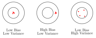
Intuition 82. Think of shooting arrows at a target:

• Low bias, low variance: Arrows cluster tightly around bullseye (ideal)

• High bias, low variance: Arrows cluster tightly, but away from bullseye (systematic error)

• Low bias, high variance: Arrows scattered around bullseye (inconsistent)

• High bias, high variance: Arrows scattered far from bullseye (worst case)

Bias-variance tradeoff visualization. Each dot represents a model trained on different data.

6.3 Model Complexity and the Tradeoff

Key Idea

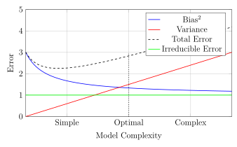
As model complexity increases:

• Bias decreases: More flexible models can fit data better

• Variance increases: More flexibility means more sensitivity to data

Sweet spot: Balance bias and variance to minimize total error.

Bias-variance tradeoff as a function of model complexity

6.4 Examples by Model Type

Bias-variance characteristics of different models

Model	Bias	Variance
Linear Regression	High (if data non-linear)	Low
High-degree Polynomial	Low	High
KNN with \(k=1\)	Low	High
KNN with large \(k\)	High	Low
Shallow Decision Tree	High	Low
Deep Decision Tree	Low	High

6.5 Controlling the Tradeoff

6.5.1 Cross-Validation

Definition 6.5 (\(k\)-Fold Cross-Validation).

1. Split data into \(k\) equal folds

2. For \(i = 1, \ldots, k\):

   • Train on folds \(\{1, \ldots, k\} \setminus \{i\}\)

   • Validate on fold \(i\)

   • Record error \(E_i\)

3. Report average: \(\text{CV Error} = \frac{1}{k}\sum_{i=1}^k E_i\)

Common choice: \(k = 5\) or \(k = 10\).

Use: Select hyperparameters (e.g., polynomial degree, regularization \(\lambda\), tree depth) by choosing the value with lowest CV error.

Definition 6.6 (Leave-One-Out Cross-Validation (LOOCV)). Special case with \(k = n\) (number of examples). Train on \(n-1\) examples, test on 1. Repeat for each example.

Pros: Maximum training data, nearly unbiased estimate

Cons: Computationally expensive (\(n\) model fits)

6.5.2 Regularization

As discussed earlier, regularization (Ridge, Lasso, ElasticNet) explicitly controls model complexity:

• Increases bias (restricts model flexibility)

• Decreases variance (less overfitting)

• Tune \(\lambda\) via cross-validation to find optimal tradeoff

6.5.3 Ensemble Methods

Preview of Part 3: Combining multiple models can reduce variance without increasing bias:

• Bagging (e.g., Random Forests): Reduces variance by averaging

• Boosting (e.g., XGBoost): Reduces bias by sequential learning

6.6 Summary of Part 1

1. Linear Regression: Foundation of supervised learning. Normal equation for closed-form; gradient descent for iterative solution.

2. Regularization: Ridge (\(\ell_2\)) for shrinkage, Lasso (\(\ell_1\)) for sparsity. Essential for high-dimensional data.

3. Logistic Regression: Linear model for classification using sigmoid function and cross-entropy loss.

4. KNN: Non-parametric, instance-based learning. Simple but suffers from curse of dimensionality.

5. Decision Trees: Interpretable, handles non-linear patterns. Prone to overfitting without pruning.

6. Bias-Variance Tradeoff: Fundamental tension in ML. Simple models: high bias, low variance. Complex models: low bias, high variance. Use cross-validation and regularization to balance.

Next Steps: Part 2 explores probabilistic models (Naive Bayes, SVMs) that provide uncertainty estimates and maximum-margin classification.

Exercise 6.7.

1. Derive the gradient of Ridge regression loss and show it leads to \(\boldsymbol{w}^* = (\boldsymbol{X}^\top\boldsymbol{X} + \lambda\boldsymbol{I})^{-1}\boldsymbol{X}^\top\boldsymbol{y}\).

2. Prove that the sigmoid derivative is \(\sigma'(z) = \sigma(z)(1-\sigma(z))\).

3. For a dataset with 8 positive and 4 negative examples, compute the entropy. If a feature splits it into (6 pos, 1 neg) and (2 pos, 3 neg), compute the information gain.

4. Implement KNN (\(k=3\)) on 2D data: \(\{(1,1,+), (2,2,+), (3,1,+), (6,5,-), (7,7,-), (8,6,-)\}\). Classify the point \((4,3)\).

5. For polynomial regression with degree \(d\), how many parameters are in the model? How does this relate to overfitting as \(d\) increases?

6. Draw a bias-variance diagram and mark where the following would fall: (a) \(k=1\) KNN, (b) Linear regression on non-linear data, (c) Deep decision tree.

Part 2: Probabilistic Models

7 Naive Bayes

7.1 Probabilistic Classification Framework

Unlike discriminative models (which learn \(P(y|\boldsymbol{x})\) directly), generative models learn the joint distribution \(P(\boldsymbol{x}, y)\) and use Bayes’ rule for prediction.

Definition 7.1 (Bayes’ Rule for Classification). Given features \(\boldsymbol{x}\) and class \(y \in \{1, 2, \ldots, K\}\): \[P(y = c | \boldsymbol{x}) = \frac{P(\boldsymbol{x} | y = c) \cdot P(y = c)}{P(\boldsymbol{x})} = \frac{P(\boldsymbol{x} | y = c) \cdot P(y = c)}{\sum_{k=1}^K P(\boldsymbol{x} | y = k) \cdot P(y = k)}\] where:

• \(P(y=c|\boldsymbol{x})\) is the posterior probability (what we want)

• \(P(\boldsymbol{x}|y=c)\) is the likelihood (how likely are these features given class \(c\))

• \(P(y=c)\) is the prior (how common is class \(c\) in general)

• \(P(\boldsymbol{x})\) is the evidence (normalization constant)

Classification rule: \[\hat{y} = \mathop{\mathrm{arg\,max}}_{c} P(y=c|\boldsymbol{x}) = \mathop{\mathrm{arg\,max}}_{c} P(\boldsymbol{x}|y=c) \cdot P(y=c)\] We can ignore \(P(\boldsymbol{x})\) since it doesn’t depend on \(c\).

7.2 The Naive Bayes Assumption

Challenge: For \(d\) features, estimating \(P(\boldsymbol{x}|y=c) = P(x_1, x_2, \ldots, x_d | y=c)\) requires exponentially many parameters.

Solution: Assume conditional independence.

Definition 7.2 (Naive Bayes Assumption). Features are conditionally independent given the class: \[P(\boldsymbol{x} | y = c) = P(x_1, x_2, \ldots, x_d | y = c) = \prod_{j=1}^d P(x_j | y = c)\]

Intuition 88. “Naive” because we assume features don’t interact given the class. For spam detection: knowing an email contains “free” doesn’t change the probability of “money” appearing, given we know it’s spam. This is often false in reality, but works surprisingly well in practice!

Theorem 7.4 (Naive Bayes Classifier). \[\hat{y} = \mathop{\mathrm{arg\,max}}_{c} P(y=c) \prod_{j=1}^d P(x_j | y=c)\] In log space (for numerical stability): \[\hat{y} = \mathop{\mathrm{arg\,max}}_{c} \left[\log P(y=c) + \sum_{j=1}^d \log P(x_j | y=c)\right]\]

7.3 Estimating Parameters

From training data \(\mathcal{D} = \{(\boldsymbol{x}_i, y_i)\}_{i=1}^n\):

Definition 7.5 (Prior Estimation). \[P(y = c) = \frac{\text{count}(y=c)}{n}\] Simply the fraction of training examples in class \(c\).

Definition 7.6 (Likelihood Estimation). Depends on the type of features:

• Categorical: \(P(x_j = v | y=c) = \frac{\text{count}(x_j=v, y=c)}{\text{count}(y=c)}\)

• Continuous: Assume a distribution (e.g., Gaussian) and estimate parameters

7.4 Variants of Naive Bayes

7.4.1 Gaussian Naive Bayes

For continuous features, assume each feature follows a Gaussian distribution.

Definition 7.7 (Gaussian Naive Bayes). Assume \(P(x_j | y=c) \sim \mathcal{N}(\mu_{jc}, \sigma_{jc}^2)\): \[P(x_j | y=c) = \frac{1}{\sqrt{2\pi\sigma_{jc}^2}} \exp\left(-\frac{(x_j - \mu_{jc})^2}{2\sigma_{jc}^2}\right)\] where \(\mu_{jc}\) and \(\sigma_{jc}^2\) are estimated from training data: \[\mu_{jc} = \frac{1}{n_c}\sum_{i: y_i=c} x_{ij}, \quad \sigma_{jc}^2 = \frac{1}{n_c}\sum_{i: y_i=c} (x_{ij} - \mu_{jc})^2\]

Example 7.8 (Medical Diagnosis). Predict disease (yes/no) from symptoms: temperature and blood pressure.

Training data:

• Disease=Yes (3 examples): temps = [38.5, 39.0, 38.7], BP = [140, 145, 142]

• Disease=No (2 examples): temps = [36.8, 37.1], BP = [120, 118]

Estimates:

• \(P(\text{Disease}=\text{Yes}) = 3/5 = 0.6\)

• \(\mu_{\text{temp,yes}} = 38.73\), \(\sigma_{\text{temp,yes}}^2 = 0.043\)

• \(\mu_{\text{temp,no}} = 36.95\), \(\sigma_{\text{temp,no}}^2 = 0.0225\)

• Similar for blood pressure

Test: Patient with temp=38.0, BP=135. Compute both posteriors and predict the larger.

7.4.2 Multinomial Naive Bayes

For count data (e.g., word frequencies in documents).

Definition 7.9 (Multinomial Naive Bayes). Each feature \(x_j\) is a count of how many times feature \(j\) appears. Model: \[P(\boldsymbol{x} | y=c) = \frac{\left(\sum_j x_j\right)!}{\prod_j x_j!} \prod_{j=1}^d \theta_{jc}^{x_j}\] where \(\theta_{jc} = P(\text{feature } j | y=c)\).

Parameter estimation (with Laplace smoothing): \[\theta_{jc} = \frac{\text{count}(x_j, y=c) + \alpha}{\sum_{j'} \text{count}(x_{j'}, y=c) + \alpha d}\] \(\alpha > 0\) is a smoothing parameter (typically \(\alpha=1\)).

Intuition 95. Laplace smoothing prevents zero probabilities. If a word never appears in spam training data, we still assign it a small non-zero probability rather than zero (which would make the entire product zero).

Example 7.11 (Text Classification). Classify documents as “sports” or “politics”.

Vocabulary: {game, team, vote, election, win}

Training:

• Sports docs: “game win”, “team game”, “team win win”

• Politics docs: “vote election”, “election win”

Word counts by class:

• Sports: game=3, team=2, vote=0, election=0, win=4

• Politics: game=0, team=0, vote=1, election=2, win=1

With \(\alpha=1\): \[\theta_{\text{game,sports}} = \frac{3+1}{9+5} = \frac{4}{14} \approx 0.286\]

Test: “game election” \(\to\) compute \(P(\text{sports}|\text{doc})\) and \(P(\text{politics}|\text{doc})\).

7.4.3 Bernoulli Naive Bayes

For binary features (presence/absence).

Definition 7.12 (Bernoulli Naive Bayes). Each \(x_j \in \{0, 1\}\) indicates feature presence: \[P(x_j | y=c) = \theta_{jc}^{x_j}(1-\theta_{jc})^{1-x_j}\] where \(\theta_{jc} = P(x_j=1 | y=c)\).

Estimation: \[\theta_{jc} = \frac{\text{count}(x_j=1, y=c) + \alpha}{\text{count}(y=c) + 2\alpha}\]

Multinomial vs Bernoulli: Multinomial uses counts; Bernoulli uses only presence/absence. For text: Bernoulli asks “Does word \(j\) appear?”; Multinomial asks “How many times?”

7.5 Applications

Key Idea

Spam Filtering:

• Features: words in email

• Classes: spam / not spam

• Use Multinomial or Bernoulli NB

• Fast training and prediction

Document Classification:

• Categorize news articles, scientific papers

• Large vocabularies: naive assumption helps reduce parameters

Sentiment Analysis:

• Classify reviews as positive/negative

• Features: word frequencies or presence

Advantages:

• Simple, fast training and prediction

• Works well with small training data

• Handles high-dimensional data naturally

• Probabilistic predictions (useful for uncertainty estimation)

Limitations:

• Strong independence assumption rarely holds

• Poor at capturing feature interactions

• Probability estimates can be extreme (overconfident)

8 Generative vs Discriminative Models

8.1 Key Distinction

Definition 8.1 (Discriminative Models). Learn the conditional probability \(P(y|\boldsymbol{x})\) directly.

Examples: Logistic regression, SVM, decision trees, neural networks

Goal: Find the decision boundary separating classes

Definition 8.2 (Generative Models). Learn the joint probability \(P(\boldsymbol{x}, y) = P(\boldsymbol{x}|y)P(y)\) and use Bayes’ rule.

Examples: Naive Bayes, Gaussian Discriminant Analysis, HMMs

Goal: Model how data is generated for each class

Generative vs discriminative models

Aspect	Generative	Discriminative
Learns	\(P(\boldsymbol{x}, y)\)	\(P(y|\boldsymbol{x})\)
Can sample new data?	Yes	No
Outlier detection	Natural	Difficult
Performance (large data)	Often worse	Often better
Performance (small data)	Often better	Often worse
Can handle missing features?	Yes (naturally)	Difficult

Intuition 100. Generative: “I understand what cats and dogs look like. Let me generate examples of each and see which your image resembles.”

Discriminative: “I just need to distinguish cats from dogs. Let me find the boundary that separates them best.”

Generative models do more (model full distribution), so they need more assumptions. Discriminative models focus only on the decision boundary, often giving better classification.

8.2 Gaussian Discriminant Analysis (GDA)

GDA is a generative classifier that models each class as a multivariate Gaussian.

Definition 8.4 (GDA Model). For binary classification (\(y \in \{0, 1\}\)): \[\begin{align} y &\sim \text{Bernoulli}(\phi) \\ \boldsymbol{x}|y=0 &\sim \mathcal{N}(\boldsymbol{\mu}_0, \boldsymbol{\Sigma}) \\ \boldsymbol{x}|y=1 &\sim \mathcal{N}(\boldsymbol{\mu}_1, \boldsymbol{\Sigma}) \end{align}\] Note: We assume the same covariance \(\boldsymbol{\Sigma}\) for both classes.

Theorem 8.5 (GDA Parameters). Maximum likelihood estimates from data \(\{(\boldsymbol{x}_i, y_i)\}_{i=1}^n\): \[\begin{align} \phi &= \frac{1}{n} \sum_{i=1}^n \mathbb{I}(y_i = 1), \\ \boldsymbol{\mu}_0 &= \frac{\sum_{i=1}^n \mathbb{I}(y_i = 0)\,\boldsymbol{x}_i}{\sum_{i=1}^n \mathbb{I}(y_i = 0)}, \\ \boldsymbol{\mu}_1 &= \frac{\sum_{i=1}^n \mathbb{I}(y_i = 1)\,\boldsymbol{x}_i}{\sum_{i=1}^n \mathbb{I}(y_i = 1)}, \\ \boldsymbol{\Sigma} &= \frac{1}{n} \sum_{i=1}^n \bigl(\boldsymbol{x}_i - \boldsymbol{\mu}_{y_i}\bigr)\bigl(\boldsymbol{x}_i - \boldsymbol{\mu}_{y_i}\bigr)^\top. \end{align}\]

Theorem 8.6 (GDA Decision Boundary). The decision boundary where \(P(y=1|\boldsymbol{x}) = P(y=0|\boldsymbol{x})\) is linear: \[\boldsymbol{w}^\top\boldsymbol{x} + w_0 = 0\] where \(\boldsymbol{w} = \boldsymbol{\Sigma}^{-1}(\boldsymbol{\mu}_1 - \boldsymbol{\mu}_0)\) and \(w_0\) involves \(\phi\), \(\boldsymbol{\mu}_0\), \(\boldsymbol{\mu}_1\).

This shows GDA produces a linear classifier, similar to logistic regression!

Key Idea

GDA vs Logistic Regression:

• Both produce linear decision boundaries

• GDA makes stronger assumptions (Gaussian distributions)

• If assumptions hold, GDA is more efficient (needs less data)

• If assumptions violated, logistic regression is more robust

• GDA can be viewed as a special case that implies logistic regression

Rule of thumb: Try both. If data looks roughly Gaussian, GDA may work better. Otherwise, prefer logistic regression.

8.3 Hidden Markov Models (Brief Overview)

Definition 8.7 (Hidden Markov Model (HMM)). A sequence model with:

• Hidden states \(z_1, z_2, \ldots, z_T\) (not observed)

• Observations \(x_1, x_2, \ldots, x_T\) (observed)

• Transition probabilities: \(P(z_t | z_{t-1})\)

• Emission probabilities: \(P(x_t | z_t)\)

Intuition 105. Think of speech recognition: hidden states are phonemes (sound units), observations are audio features. We observe the audio but want to infer the underlying phoneme sequence.

Key algorithms:

• Forward-Backward: Compute \(P(\boldsymbol{x})\) (likelihood)

• Viterbi: Find most likely hidden state sequence \(\mathop{\mathrm{arg\,max}}_{\boldsymbol{z}} P(\boldsymbol{z}|\boldsymbol{x})\)

• Baum-Welch: Learn parameters (EM algorithm)

Applications: Speech recognition, part-of-speech tagging, bioinformatics (gene prediction).

Remark 106. HMMs are beyond the scope of this introductory treatment. They represent an important class of generative models for sequential data. Modern alternatives include RNNs and Transformers (covered in Part 4).

9 Support Vector Machines

9.1 Intuition: Maximum Margin Classification

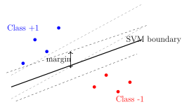
Unlike logistic regression (which finds any separating hyperplane), SVM finds the hyperplane with the largest margin.

Definition 9.1 (Margin). The margin is the distance from the decision boundary to the nearest data point.

A maximum margin classifier maximizes this distance.

Intuition 108. Imagine two classes of points that are linearly separable. Many hyperplanes separate them, but intuitively, the one in the “middle” (farthest from both classes) is most robust to noise and generalizes better.

SVM finds the hyperplane with maximum margin (thick line) between classes

9.2 Mathematical Formulation (Hard Margin)

Definition 9.3 (Linear Classifier). Decision function: \(f(\boldsymbol{x}) = \boldsymbol{w}^\top\boldsymbol{x} + b\)

Prediction: \(\hat{y} = \text{sign}(f(\boldsymbol{x})) = \begin{cases} +1 & \text{if } f(\boldsymbol{x}) > 0 \\ -1 & \text{if } f(\boldsymbol{x}) < 0 \end{cases}\)

Definition 9.4 (Functional and Geometric Margin). Functional margin of \((\boldsymbol{w}, b)\) with respect to \((\boldsymbol{x}_i, y_i)\): \[\hat{\gamma}_i = y_i(\boldsymbol{w}^\top\boldsymbol{x}_i + b)\] Positive when correctly classified.

Geometric margin (actual distance to hyperplane): \[\gamma_i = \frac{y_i(\boldsymbol{w}^\top\boldsymbol{x}_i + b)}{\left\lVert\boldsymbol{w}\right\rVert}\]

Theorem 9.5 (Hard Margin SVM (Primal Form)). To maximize the margin: \[\begin{aligned} \max_{\boldsymbol{w}, b} \quad & \frac{1}{\left\lVert\boldsymbol{w}\right\rVert} \\ \text{subject to} \quad & y_i(\boldsymbol{w}^\top\boldsymbol{x}_i + b) \geq 1, \quad i = 1, \ldots, n \end{aligned}\] Equivalently (minimization form): \[\begin{aligned} \min_{\boldsymbol{w}, b} \quad & \frac{1}{2}\left\lVert\boldsymbol{w}\right\rVert^2 \\ \text{subject to} \quad & y_i(\boldsymbol{w}^\top\boldsymbol{x}_i + b) \geq 1, \quad i = 1, \ldots, n \end{aligned}\]

Intuition 112. The constraint \(y_i(\boldsymbol{w}^\top\boldsymbol{x}_i + b) \geq 1\) ensures all points are correctly classified and at least distance \(1/\left\lVert\boldsymbol{w}\right\rVert\) from the boundary. Minimizing \(\left\lVert\boldsymbol{w}\right\rVert^2\) maximizes the margin \(1/\left\lVert\boldsymbol{w}\right\rVert\).

9.3 Lagrange Duality and the Dual Form

The primal is a constrained optimization problem. We use Lagrange multipliers.

Definition 9.7 (Lagrangian). \[\mathcal{L}(\boldsymbol{w}, b, \boldsymbol{\alpha}) = \frac{1}{2}\left\lVert\boldsymbol{w}\right\rVert^2 - \sum_{i=1}^n \alpha_i[y_i(\boldsymbol{w}^\top\boldsymbol{x}_i + b) - 1]\] where \(\alpha_i \geq 0\) are Lagrange multipliers.

Theorem 9.8 (KKT Conditions). At the optimum:

1. \(\nabla_{\boldsymbol{w}} \mathcal{L} = 0 \implies \boldsymbol{w} = \sum_{i=1}^n \alpha_i y_i \boldsymbol{x}_i\)

2. \(\frac{\partial \mathcal{L}}{\partial b} = 0 \implies \sum_{i=1}^n \alpha_i y_i = 0\)

3. \(\alpha_i \geq 0\)

4. \(\alpha_i [y_i(\boldsymbol{w}^\top\boldsymbol{x}_i + b) - 1] = 0\) (complementary slackness)

Key Idea

The complementary slackness condition is crucial:

• If \(\alpha_i > 0\), then \(y_i(\boldsymbol{w}^\top\boldsymbol{x}_i + b) = 1\) (point is on the margin)

• These points are called support vectors

• Only support vectors affect the decision boundary!

• Most \(\alpha_i = 0\) \(\to\) sparse solution

Theorem 9.9 (Dual Form). Substituting the KKT conditions into the Lagrangian: \[\begin{aligned} \max_{\boldsymbol{\alpha}} \quad & \sum_{i=1}^n \alpha_i - \frac{1}{2}\sum_{i=1}^n\sum_{j=1}^n \alpha_i\alpha_j y_i y_j \boldsymbol{x}_i^\top\boldsymbol{x}_j \\ \text{subject to} \quad & \alpha_i \geq 0, \quad i = 1, \ldots, n \\ & \sum_{i=1}^n \alpha_i y_i = 0 \end{aligned}\] This is a quadratic programming problem in \(\boldsymbol{\alpha}\).

Why dual is useful:

• Only depends on dot products \(\boldsymbol{x}_i^\top\boldsymbol{x}_j\) (enables kernel trick!)

• Sparse solution (most \(\alpha_i = 0\))

• Once solved, prediction: \(f(\boldsymbol{x}) = \sum_{i=1}^n \alpha_i y_i \boldsymbol{x}_i^\top\boldsymbol{x} + b\)

9.4 The Kernel Trick

Problem: What if data is not linearly separable?

Solution: Map data to higher-dimensional space where it becomes separable!

Definition 9.10 (Feature Map). Let \(\boldsymbol{\phi}: \mathbb{R}^d \to \mathbb{R}^D\) (with \(D \gg d\)) be a feature map.

Transform: \(\boldsymbol{x} \to \boldsymbol{\phi}(\boldsymbol{x})\)

Run SVM in the transformed space: \(f(\boldsymbol{x}) = \boldsymbol{w}^\top\boldsymbol{\phi}(\boldsymbol{x}) + b\)

Example 9.11 (Simple Kernel). For \(\boldsymbol{x} = [x_1, x_2]^\top\), define: \[\boldsymbol{\phi}(\boldsymbol{x}) = [x_1^2, \sqrt{2}x_1x_2, x_2^2, \sqrt{2}x_1, \sqrt{2}x_2, 1]^\top\] This maps 2D to 6D. Data that’s not linearly separable in 2D might be in 6D!

Issue: Computing \(\boldsymbol{\phi}(\boldsymbol{x})\) explicitly for high \(D\) is expensive.

Theorem 9.12 (Kernel Trick). We only need dot products \(\boldsymbol{\phi}(\boldsymbol{x}_i)^\top\boldsymbol{\phi}(\boldsymbol{x}_j)\) in the dual.

Define kernel function: \(K(\boldsymbol{x}_i, \boldsymbol{x}_j) = \boldsymbol{\phi}(\boldsymbol{x}_i)^\top\boldsymbol{\phi}(\boldsymbol{x}_j)\)

If we can compute \(K\) directly without computing \(\boldsymbol{\phi}\) explicitly, we get efficiency!

Definition 9.13 (Common Kernels).

• Linear: \(K(\boldsymbol{x}, \boldsymbol{z}) = \boldsymbol{x}^\top\boldsymbol{z}\)

• Polynomial: \(K(\boldsymbol{x}, \boldsymbol{z}) = (\boldsymbol{x}^\top\boldsymbol{z} + c)^p\)

  Corresponds to all polynomials up to degree \(p\).

• RBF (Radial Basis Function / Gaussian): \[K(\boldsymbol{x}, \boldsymbol{z}) = \exp\left(-\gamma\left\lVert\boldsymbol{x} - \boldsymbol{z}\right\rVert^2\right)\] where \(\gamma > 0\) is a bandwidth parameter.

  This corresponds to infinite-dimensional feature space!

• Sigmoid: \(K(\boldsymbol{x}, \boldsymbol{z}) = \tanh(\alpha \boldsymbol{x}^\top\boldsymbol{z} + c)\)

Key Idea

The kernel trick magic:

The polynomial kernel \((x^\top z + 1)^2\) computes the dot product in a space of all degree-2 polynomials: \[(x^\top z + 1)^2 = (x_1z_1 + x_2z_2 + 1)^2 = x_1^2z_1^2 + 2x_1x_2z_1z_2 + x_2^2z_2^2 + 2x_1z_1 + 2x_2z_2 + 1\] This equals \(\boldsymbol{\phi}(\boldsymbol{x})^\top\boldsymbol{\phi}(\boldsymbol{z})\) with \(\boldsymbol{\phi}(\boldsymbol{x}) = [x_1^2, \sqrt{2}x_1x_2, x_2^2, \sqrt{2}x_1, \sqrt{2}x_2, 1]^\top\).

We computed this in \(O(d)\) time instead of \(O(D)\) where \(D=\binom{d+2}{2}\)!

For RBF kernel: we operate in infinite dimensions without ever computing infinite-dimensional vectors!

Theorem 9.14 (Kernelized Dual). With kernel \(K\): \[\begin{aligned} \max_{\boldsymbol{\alpha}} \quad & \sum_{i=1}^n \alpha_i - \frac{1}{2}\sum_{i=1}^n\sum_{j=1}^n \alpha_i\alpha_j y_i y_j K(\boldsymbol{x}_i, \boldsymbol{x}_j) \\ \text{subject to} \quad & \alpha_i \geq 0, \sum_{i=1}^n \alpha_i y_i = 0 \end{aligned}\] Prediction: \(f(\boldsymbol{x}) = \sum_{i=1}^n \alpha_i y_i K(\boldsymbol{x}_i, \boldsymbol{x}) + b\)

9.5 Soft Margin SVM

Problem: Real data is rarely perfectly separable. Hard margin SVM fails if any point violates the constraint.

Solution: Allow some misclassifications with penalty.

Definition 9.15 (Slack Variables). Introduce \(\xi_i \geq 0\) for each point:

• \(\xi_i = 0\): Point correctly classified with margin \(\geq 1\)

• \(0 < \xi_i < 1\): Correctly classified but within margin

• \(\xi_i \geq 1\): Misclassified

Relaxed constraint: \(y_i(\boldsymbol{w}^\top\boldsymbol{x}_i + b) \geq 1 - \xi_i\)

Theorem 9.16 (Soft Margin SVM). \[\begin{aligned} \min_{\boldsymbol{w}, b, \boldsymbol{\xi}} \quad & \frac{1}{2}\left\lVert\boldsymbol{w}\right\rVert^2 + C\sum_{i=1}^n \xi_i \\ \text{subject to} \quad & y_i(\boldsymbol{w}^\top\boldsymbol{x}_i + b) \geq 1 - \xi_i \\ & \xi_i \geq 0, \quad i = 1, \ldots, n \end{aligned}\] \(C > 0\) is a hyperparameter controlling the trade-off:

• Large \(C\): Fewer violations allowed (closer to hard margin, may overfit)

• Small \(C\): More violations allowed (more regularization, may underfit)

Intuition 123. Soft margin balances two goals:

1. Maximize margin (minimize \(\left\lVert\boldsymbol{w}\right\rVert^2\))

2. Minimize classification errors (minimize \(\sum \xi_i\))

Parameter \(C\) controls this trade-off. Use cross-validation to choose \(C\).

Definition 9.18 (Hinge Loss Formulation). Soft margin SVM can be written as: \[\min_{\boldsymbol{w}, b} \frac{1}{2}\left\lVert\boldsymbol{w}\right\rVert^2 + C\sum_{i=1}^n \max(0, 1 - y_i(\boldsymbol{w}^\top\boldsymbol{x}_i + b))\] where \(\ell_{\text{hinge}}(z) = \max(0, 1-z)\) is the hinge loss.

This connects SVM to other loss functions (logistic loss, squared loss, etc.).

9.6 Support Vector Regression (SVR)

SVM can also be used for regression!

Definition 9.19 (\(\epsilon\)-insensitive Loss). \[\ell_\epsilon(y, \hat{y}) = \begin{cases} 0 & \text{if } |y - \hat{y}| < \epsilon \\ |y - \hat{y}| - \epsilon & \text{otherwise} \end{cases}\] No penalty for predictions within \(\epsilon\) of the true value.

Definition 9.20 (SVR Formulation). \[\begin{aligned} \min_{\boldsymbol{w}, b} \quad & \frac{1}{2}\left\lVert\boldsymbol{w}\right\rVert^2 + C\sum_{i=1}^n (\xi_i + \xi_i^*)\\ \text{subject to} \quad & y_i - (\boldsymbol{w}^\top\boldsymbol{x}_i + b) \leq \epsilon + \xi_i \\ & (\boldsymbol{w}^\top\boldsymbol{x}_i + b) - y_i \leq \epsilon + \xi_i^* \\ & \xi_i, \xi_i^* \geq 0 \end{aligned}\]

Intuition 127. SVR fits a “tube” of width \(2\epsilon\) around the data. Points inside the tube have no penalty. Points outside pay a linear penalty proportional to their distance from the tube.

9.7 Practical Considerations

Implementation Notes

Choosing SVM Parameters:

• Kernel: Start with RBF (most flexible). Try linear if \(d\) is large.

• \(C\): Controls regularization. Use grid search + CV.

• \(\gamma\) (for RBF): Controls kernel width. Small \(\gamma\) = wide kernel (smooth), large \(\gamma\) = narrow kernel (complex boundary).

Feature Scaling: Critical for SVMs! Since they use distances, features should be normalized (e.g., to \([0,1]\) or standardized to mean 0, std 1).

Complexity:

• Training: \(O(n^2 d)\) to \(O(n^3)\) (solving QP)

• Prediction: \(O(n_{\text{sv}} d)\) where \(n_{\text{sv}}\) is number of support vectors

When to use SVMs:

• Medium-sized datasets (1000s to 100,000s of examples)

• High-dimensional data (works well when \(d > n\))

• When you need a strong theoretical guarantee (maximum margin)

• Non-linear decision boundaries (with kernels)

When NOT to use SVMs:

• Very large datasets (\(n > 1\)M) - use linear models or neural networks

• When interpretability is critical - use decision trees or linear models

• When probabilistic outputs are essential - use logistic regression or Naive Bayes

9.8 Summary of Part 2

1. Naive Bayes: Generative classifier using Bayes’ rule with conditional independence assumption. Fast, works well for text classification despite “naive” assumption.

2. Generative vs Discriminative: Generative models (\(P(\boldsymbol{x}, y)\)) model how data is generated; discriminative models (\(P(y|\boldsymbol{x})\)) focus on decision boundaries. Trade-offs in performance, data requirements, and capabilities.

3. GDA: Assumes Gaussian distributions per class. Produces linear boundaries like logistic regression but with stronger assumptions.

4. SVM: Maximum margin classifier. Primal form maximizes margin; dual form enables kernel trick. Soft margin allows violations with penalty \(C\).

5. Kernel Trick: Implicitly maps to high (or infinite) dimensional spaces via kernel functions. RBF kernel most popular for non-linear boundaries.

6. SVR: Adapts SVM for regression using \(\epsilon\)-insensitive loss. Fits tube around data.

Next Steps: Part 3 explores ensemble methods (Bagging, Boosting, Stacking) that combine multiple models to achieve better performance than any single model.

Exercise 9.22.

1. Given training data for spam (words: “free”=10, “money”=8) and ham (“free”=2, “money”=1), with priors \(P(\text{spam})=0.4\), compute \(P(\text{spam}|\text{``free money''})\) using Multinomial Naive Bayes with Laplace smoothing (\(\alpha=1\)).

2. Prove that if we assume Gaussian distributions with same covariance for both classes (GDA), the posterior \(P(y=1|\boldsymbol{x})\) has the form of logistic regression.

3. For the polynomial kernel \(K(\boldsymbol{x}, \boldsymbol{z}) = (\boldsymbol{x}^\top\boldsymbol{z} + 1)^2\), explicitly write out the feature map \(\boldsymbol{\phi}(\boldsymbol{x})\) for \(\boldsymbol{x} \in \mathbb{R}^2\).

4. Show that the RBF kernel \(K(\boldsymbol{x}, \boldsymbol{z}) = \exp(-\gamma\left\lVert\boldsymbol{x}-\boldsymbol{z}\right\rVert^2)\) satisfies the property \(K(\boldsymbol{x}, \boldsymbol{x}) = 1\) and \(K(\boldsymbol{x}, \boldsymbol{z}) \to 0\) as \(\left\lVert\boldsymbol{x}-\boldsymbol{z}\right\rVert \to \infty\).

5. Consider a 1D SVM with data \(\{(1, +1), (2, +1), (4, -1), (5, -1)\}\). Assuming hard margin is feasible, what are the support vectors?

6. Explain why feature scaling is critical for SVMs but not for decision trees.

Part 3: Ensemble Methods

10 Introduction to Ensemble Learning

Definition 10.1 (Ensemble Learning). An ensemble method combines predictions from multiple base models (called learners or weak learners) to produce a final prediction that is typically more accurate and robust than any individual model.

Intuition 130. “Wisdom of crowds”: Just as a group of people can make better decisions than individuals, combining multiple models can reduce errors. Different models make different mistakes; by aggregating, we can cancel out individual errors.

Key Idea

Why Ensembles Work:

From the bias-variance perspective:

• Reduce Variance: Average multiple high-variance models (e.g., deep trees) \(\to\) more stable predictions

• Reduce Bias: Sequentially build models that correct errors of previous ones \(\to\) better fit

• Improve Robustness: Different models capture different patterns; ensemble is less likely to fail

Three Main Paradigms:

1. Bagging: Train models independently on bootstrap samples, then average (reduces variance)

2. Boosting: Train models sequentially, each focusing on previous errors (reduces bias)

3. Stacking: Train a meta-model to combine base model predictions (learns optimal combination)

11 Bagging (Bootstrap Aggregating)

11.1 Bootstrap Sampling

Definition 11.1 (Bootstrap Sample). Given a dataset \(\mathcal{D}\) of size \(n\), a bootstrap sample \(\mathcal{D}_i\) is created by:

1. Randomly sample \(n\) examples from \(\mathcal{D}\) with replacement

2. Some examples appear multiple times, others not at all

On average, about 63.2% of unique examples appear in each bootstrap sample.

Why 63.2%?. Probability that example \(i\) is NOT selected in one draw: \((1 - 1/n)\)

Probability NOT selected in \(n\) draws: \((1 - 1/n)^n\)

As \(n \to \infty\): \((1 - 1/n)^n \to e^{-1} \approx 0.368\)

So probability of being selected: \(1 - 0.368 = 0.632\) or 63.2%. ◻

11.2 Bagging Algorithm

Algorithm Summary

Bagging for Classification/Regression

Input:

• Training data \(\mathcal{D} = \{(\boldsymbol{x}_i, y_i)\}_{i=1}^n\)

• Base learning algorithm \(\mathcal{A}\)

• Number of models \(M\)

Training:

1. For \(m = 1\) to \(M\):

   • Create bootstrap sample \(\mathcal{D}_m\) by sampling \(n\) examples from \(\mathcal{D}\) with replacement

   • Train base learner: \(h_m = \mathcal{A}(\mathcal{D}_m)\)

Prediction for new example \(\boldsymbol{x}\):

• Classification: \(\hat{y} = \text{majority\_vote}(h_1(\boldsymbol{x}), h_2(\boldsymbol{x}), \ldots, h_M(\boldsymbol{x}))\)

• Regression: \(\hat{y} = \frac{1}{M}\sum_{m=1}^M h_m(\boldsymbol{x})\)

Output: Ensemble predictor \(H(\boldsymbol{x})\)

Theorem 11.2 (Variance Reduction in Bagging). Suppose we have \(M\) independent models, each with variance \(\sigma^2\) and we average their predictions. The variance of the ensemble is: \[\mathrm{Var}(\text{average}) = \frac{\sigma^2}{M}\] If models are correlated with correlation \(\rho\): \[\mathrm{Var}(\text{average}) = \rho\sigma^2 + \frac{1-\rho}{M}\sigma^2\] As \(M \to \infty\), variance approaches \(\rho\sigma^2\).

Key Idea

Bagging reduces variance most when:

1. Base learners have high variance (e.g., deep decision trees)

2. Base learners are diverse (low correlation \(\rho\))

This is why bagging works best with unstable algorithms like decision trees, but doesn’t help much with stable algorithms like linear regression.

11.3 Random Forests

Random Forests extend bagging by adding another source of randomness.

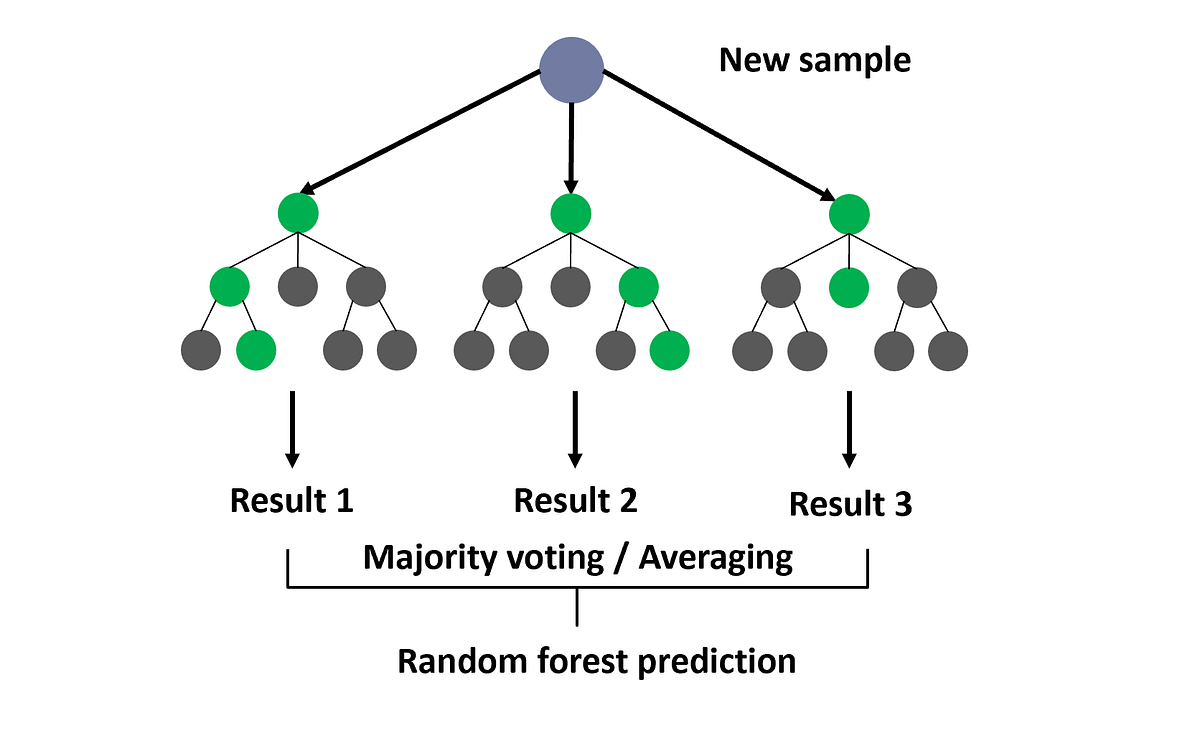
Definition 11.3 (Random Forest). A Random Forest is an ensemble of decision trees where:

1. Each tree is trained on a bootstrap sample (like bagging)

2. Additional randomness: At each split, only a random subset of \(m\) features is considered (out of total \(d\) features)

Feature subset size \(m\):

• Classification: \(m = \lfloor\sqrt{d}\rfloor\) (default)

• Regression: \(m = \lfloor d/3 \rfloor\) (default)

• Can tune via cross-validation

Intuition 134. Why limit features at each split?

Without this, trees in bagging would be similar—they’d all split on the strongest features first. By randomly limiting choices, we force trees to consider different features, increasing diversity and decorrelating predictions.

Algorithm Summary

Random Forest Algorithm

Input: Data \(\mathcal{D}\), number of trees \(M\), feature subset size \(m\)

For \(i = 1\) to \(M\):

1. Draw bootstrap sample \(\mathcal{D}_i\) from \(\mathcal{D}\)

2. Grow tree \(T_i\) on \(\mathcal{D}_i\):

   • At each node, randomly select \(m\) features from \(d\) total

   • Choose best split among these \(m\) features only

   • Split and recurse until stopping criterion

   • Do NOT prune trees (grow to maximum depth or min samples)

Prediction: Average (regression) or vote (classification) across all \(M\) trees.

Random Forest: Multiple diverse trees vote for final prediction

11.4 Out-of-Bag (OOB) Error Estimation

Definition 11.5 (Out-of-Bag (OOB) Examples). For each bootstrap sample, approximately 37% of examples are not selected. These are called out-of-bag (OOB) examples for that tree.

For each data point \((\boldsymbol{x}_i, y_i)\), consider only trees where \(i\) was OOB. Average their predictions to get OOB prediction for \(\boldsymbol{x}_i\).

Definition 11.6 (OOB Error). \[\text{OOB Error} = \frac{1}{n}\sum_{i=1}^n \ell(y_i, \hat{y}_i^{\text{OOB}})\] where \(\hat{y}_i^{\text{OOB}}\) is the prediction using only trees where \(i\) was OOB.

Key Idea

OOB error provides a free validation estimate!

• No need for separate validation set

• Each example has been tested on \(\approx 37\%\) of trees

• Approximates cross-validation error

• Can use to tune hyperparameters (number of trees, max depth, etc.)

This is a major practical advantage of Random Forests.

11.5 Feature Importance in Random Forests

Definition 11.7 (Mean Decrease in Impurity (MDI)). For each feature \(j\), compute the total reduction in impurity (Gini or entropy) when splitting on feature \(j\), averaged over all trees and all nodes.

Higher values indicate more important features.

Definition 11.8 (Permutation Importance).

1. Compute baseline OOB error

2. For each feature \(j\):

   • Randomly permute feature \(j\) in OOB data

   • Compute new OOB error

   • Importance = increase in error

If permuting a feature greatly increases error, that feature is important.

11.6 Advantages and Limitations

Key Idea

Advantages of Random Forests:

• Excellent performance: Often among the best off-the-shelf algorithms

• Minimal tuning: Works well with default parameters

• Robust to overfitting: Even with many trees

• Handles mixed data: Numerical and categorical features

• Feature importance: Built-in importance measures

• Parallelizable: Trees trained independently

• OOB error: Free validation estimate

Limitations:

• Less interpretable: Cannot visualize like a single tree

• Memory intensive: Must store \(M\) trees

• Slow prediction: Must query \(M\) trees

• Extrapolation: Cannot predict beyond training range (averaging effect)

• Biased toward categorical features: With many levels

Typical hyperparameters:

• Number of trees \(M\): 100-1000 (more is usually better, diminishing returns)

• Max features \(m\): \(\sqrt{d}\) for classification, \(d/3\) for regression

• Min samples per leaf: 1-10 (larger = more regularization)

• Max depth: Usually unlimited (full trees)

12 Boosting

12.1 Boosting Philosophy

Unlike bagging (parallel training), boosting trains models sequentially, with each new model focusing on examples that previous models got wrong.

Intuition 139. Think of boosting as learning from mistakes:

1. Train model 1 on data

2. Identify examples model 1 struggles with

3. Train model 2 to focus on those hard examples

4. Combine models 1 and 2

5. Repeat, always focusing on current ensemble’s weaknesses

This reduces bias by creating increasingly complex models that fit the data better.

12.2 AdaBoost (Adaptive Boosting)

AdaBoost adjusts weights on training examples, increasing weights on misclassified examples.

Algorithm Summary

AdaBoost for Binary Classification

Input: Data \(\{(\boldsymbol{x}_i, y_i)\}_{i=1}^n\) with \(y_i \in \{-1, +1\}\), number of rounds \(T\)

Initialize: Weights \(w_i^{(1)} = 1/n\) for all \(i\)

For \(t = 1\) to \(T\):

1. Train weak classifier \(h_t\) on weighted data (minimizing weighted error): \[\epsilon_t = \sum_{i=1}^n w_i^{(t)} \,\mathbb{I}\bigl(h_t(\boldsymbol{x}_i) \neq y_i\bigr)\]

2. Compute classifier weight: \[\alpha_t = \frac{1}{2}\ln\left(\frac{1-\epsilon_t}{\epsilon_t}\right)\] Higher \(\alpha_t\) for more accurate classifiers.

3. Update example weights: \[w_i^{(t+1)} = w_i^{(t)} \cdot \exp(-\alpha_t y_i h_t(\boldsymbol{x}_i))\]

   • If correct (\(y_i = h_t(\boldsymbol{x}_i)\)): weight decreases

   • If incorrect (\(y_i \neq h_t(\boldsymbol{x}_i)\)): weight increases

4. Normalize: \(w_i^{(t+1)} = w_i^{(t+1)} / \sum_j w_j^{(t+1)}\)

Final classifier: \[H(\boldsymbol{x}) = \text{sign}\left(\sum_{t=1}^T \alpha_t h_t(\boldsymbol{x})\right)\]

Example 12.2 (AdaBoost Iteration). Suppose after round 1:

• Examples 1,2,3 correctly classified

• Example 4 misclassified

In round 2:

• Example 4 has much higher weight

• Next classifier focuses on getting example 4 right

• May sacrifice accuracy on 1,2,3 (which already work)

Final ensemble combines both classifiers, each weighted by \(\alpha_t\).

Theorem 12.3 (AdaBoost Training Error Bound). The training error of AdaBoost is bounded by: \[\frac{1}{n}\sum_{i=1}^n \mathbb{I}\bigl(H(\boldsymbol{x}_i) \neq y_i\bigr) \;\leq\; \prod_{t=1}^T 2\sqrt{\epsilon_t(1-\epsilon_t)}\] If each weak learner has error \(\epsilon_t \leq 1/2 - \gamma\) (better than random), then training error decreases exponentially in \(T\).

Key Idea

Weak Learner Assumption: AdaBoost requires weak learners to be better than random guessing (\(\epsilon_t < 0.5\)). Even slightly better than random is enough!

Common weak learners:

• Decision stumps: Trees with depth 1 (one split)

• Shallow trees: Depth 2-5

Why AdaBoost works:

• Reduces both bias (sequential improvement) and variance (averaging)

• Focuses on hard examples

• Adaptive weights ensure all examples eventually learned

Potential issue: Sensitive to noise and outliers (keeps increasing their weights).

12.3 Gradient Boosting

Gradient Boosting generalizes boosting to arbitrary differentiable loss functions using gradient descent in function space.

Definition 12.4 (Gradient Boosting Framework). Goal: Minimize loss over training data: \[\mathcal{L}= \sum_{i=1}^n \ell(y_i, F(\boldsymbol{x}_i))\] where \(F(\boldsymbol{x})\) is our ensemble model.

Key insight: At iteration \(t\), we have current model \(F_{t-1}\). To improve, we want to move in the direction of steepest descent: \[-\nabla_F \mathcal{L}= -\left[\frac{\partial \ell(y_i, F(\boldsymbol{x}_i))}{\partial F(\boldsymbol{x}_i)}\right]_{F=F_{t-1}}\] These are the negative gradients or pseudo-residuals.

Algorithm Summary

Gradient Boosting Machine (GBM)

Input: Data \(\{(\boldsymbol{x}_i, y_i)\}\), loss \(\ell\), number of iterations \(M\), learning rate \(\eta\)

Initialize: \(F_0(\boldsymbol{x}) = \mathop{\mathrm{arg\,min}}_c \sum_{i=1}^n \ell(y_i, c)\)

For \(m = 1\) to \(M\):

1. Compute pseudo-residuals: \[r_{im} = -\left[\frac{\partial \ell(y_i, F(\boldsymbol{x}_i))}{\partial F(\boldsymbol{x}_i)}\right]_{F=F_{m-1}}\]

2. Fit base learner \(h_m\) to pseudo-residuals: \(h_m \approx \{(\boldsymbol{x}_i, r_{im})\}\)

3. Find optimal step size: \[\rho_m = \mathop{\mathrm{arg\,min}}_\rho \sum_{i=1}^n \ell(y_i, F_{m-1}(\boldsymbol{x}_i) + \rho h_m(\boldsymbol{x}_i))\]

4. Update model: \[F_m(\boldsymbol{x}) = F_{m-1}(\boldsymbol{x}) + \eta \rho_m h_m(\boldsymbol{x})\] where \(\eta\) is the learning rate (typically 0.01-0.3).

Output: \(F_M(\boldsymbol{x})\)

Example 12.5 (Gradient Boosting for Regression). For squared loss \(\ell(y, F) = \frac{1}{2}(y - F)^2\): \[r_{im} = -\frac{\partial }{\partial F}\left[\frac{1}{2}(y_i - F)^2\right]_{F=F_{m-1}} = y_i - F_{m-1}(\boldsymbol{x}_i)\] The pseudo-residuals are just the ordinary residuals!

So Gradient Boosting for regression fits each new tree to the residuals of the current ensemble.

Key Idea

Gradient Boosting vs AdaBoost:

• AdaBoost: Adjusts example weights (specific to exponential loss)

• Gradient Boosting: Works with any differentiable loss function

Common loss functions:

• Regression: Squared loss, absolute loss, Huber loss

• Classification: Logistic loss (log-likelihood)

• Ranking: Pairwise ranking loss

Base learners: Typically shallow decision trees (depth 3-8). Deeper trees capture interactions but may overfit.

12.4 XGBoost (Extreme Gradient Boosting)

XGBoost is an optimized implementation of gradient boosting with several enhancements.

Definition 12.6 (XGBoost Objective). At iteration \(t\), minimize: \[\mathcal{L}^{(t)} = \sum_{i=1}^n \ell(y_i, F_{t-1}(\boldsymbol{x}_i) + h_t(\boldsymbol{x}_i)) + \Omega(h_t)\] where \(\Omega(h_t)\) is a regularization term: \[\Omega(h) = \gamma T + \frac{1}{2}\lambda\sum_{j=1}^T w_j^2\] \(T\) = number of leaves, \(w_j\) = leaf weights, \(\gamma\) and \(\lambda\) are regularization parameters.

Key innovations in XGBoost:

1. Regularization: Explicit control of tree complexity

2. Second-order approximation: Uses both gradients and Hessians for better optimization

3. Sparsity awareness: Handles missing values naturally

4. Column subsampling: Like Random Forest feature randomness

5. Parallel tree construction: Fast implementation

6. Cache-aware access patterns: Optimized for modern hardware

Implementation Notes

Key XGBoost Hyperparameters:

• n_estimators: Number of boosting rounds (100-1000)

• learning_rate (\(\eta\)): Step size shrinkage (0.01-0.3). Lower \(\to\) more rounds needed but better generalization

• max_depth: Tree depth (3-10). Deeper \(\to\) more interactions but overfitting

• subsample: Fraction of samples per tree (0.5-1.0). Like bootstrap in bagging

• colsample_bytree: Fraction of features per tree (0.5-1.0)

• gamma: Minimum loss reduction for split (regularization)

• lambda: L2 regularization on weights

• alpha: L1 regularization on weights

Tuning strategy:

1. Fix learning rate (e.g., 0.1), tune tree parameters (max_depth, subsample, colsample)

2. Tune regularization (gamma, lambda, alpha)

3. Lower learning rate and increase n_estimators for final model

12.5 LightGBM and CatBoost

Definition 12.7 (LightGBM). Microsoft’s gradient boosting framework with novel algorithms:

• Leaf-wise tree growth: Splits leaf with maximum gain (vs level-wise in XGBoost). Faster but can overfit—control with max_depth.

• Gradient-based One-Side Sampling (GOSS): Keeps all large-gradient examples, randomly samples small-gradient ones. Reduces data size while maintaining accuracy.

• Exclusive Feature Bundling (EFB): Bundles mutually exclusive features (sparse features). Reduces dimensionality.

Advantage: Very fast training, especially on large datasets and high dimensions.

Definition 12.8 (CatBoost). Yandex’s gradient boosting with focus on categorical features:

• Ordered boosting: Novel approach to prevent target leakage and prediction shift

• Optimal quantization: Better binning of continuous features

• Native categorical feature support: No need for manual encoding

• Symmetric trees: All trees are balanced (oblivious decision trees)

Advantage: Robust to overfitting, works well out-of-the-box, excellent for categorical data.

Comparison of modern gradient boosting implementations

Feature	XGBoost	LightGBM	CatBoost
Speed	Good	Excellent	Good
Accuracy	Excellent	Excellent	Excellent
Categorical features	Manual encoding	Manual encoding	Native support
Tree growth	Level-wise	Leaf-wise	Symmetric
Memory usage	Moderate	Low	Moderate
Overfitting resistance	Good	Moderate	Excellent
Large datasets	Good	Excellent	Good

12.6 Regularization in Boosting

Key Idea

Boosting is prone to overfitting as we add more trees. Several regularization techniques:

1. Learning Rate (Shrinkage): \[F_m = F_{m-1} + \eta \cdot h_m, \quad 0 < \eta \leq 1\] Smaller \(\eta\) requires more trees but generalizes better. Typical: \(\eta = 0.01\) to \(0.1\).

2. Early Stopping: Monitor validation error. Stop adding trees when validation error stops improving.

3. Subsampling:

• Row subsampling: Use random fraction of examples per tree (0.5-1.0)

• Column subsampling: Use random fraction of features per tree (0.5-1.0)

Adds randomness like Random Forest, reduces overfitting.

4. Tree Constraints:

• Max depth: Limit tree complexity (3-8 typically)

• Min samples per leaf: Require minimum examples in leaf nodes

• Max number of leaves: Direct control on tree size

5. Explicit Regularization (XGBoost): Add penalty terms for tree complexity (number of leaves, L1/L2 on weights).

Best practice: Combine multiple techniques. Use cross-validation to tune.

12.7 When to Use Boosting vs Bagging

Bagging vs Boosting comparison

Criterion	Bagging (Random Forest)	Boosting (XGBoost/GBM)
Primary goal	Reduce variance	Reduce bias
Training	Parallel (fast)	Sequential (slower)
Overfitting risk	Low	Moderate to high
Tuning required	Minimal	Significant
Interpretability	Low	Very low
Robustness to noise	High	Moderate (sensitive)
Small datasets	Good	Excellent
Large datasets	Excellent	Good
Out-of-box performance	Very good	Good (needs tuning)
Best accuracy (tuned)	Excellent	Excellent

Rule of thumb:

• Start with Random Forest (robust, minimal tuning)

• If need last few % accuracy and have time to tune: try XGBoost/LightGBM

• If have categorical features: consider CatBoost

• If have outliers/noise: prefer Random Forest

• For Kaggle competitions: ensemble of both often wins!

13 Stacking and Blending

13.1 Stacking (Stacked Generalization)

Definition 13.1 (Stacking). Train a meta-model (or blender) to combine predictions from multiple base models.

Two levels:

1. Level 0: Train diverse base models on training data

2. Level 1: Train meta-model on base model predictions

Algorithm Summary

Stacking with Cross-Validation

Training:

Step 1: Train level-0 models with CV

1. Split training data into \(K\) folds

2. For each base model \(m\) and fold \(k\):

   • Train \(m\) on folds \(\{1, \ldots, K\} \setminus \{k\}\)

   • Predict on fold \(k\) (out-of-fold predictions)

3. Concatenate out-of-fold predictions to get \(\hat{\boldsymbol{y}}_m^{\text{OOF}}\) for each model

4. Retrain each model on full training set for final level-0 models

Step 2: Train level-1 meta-model

• Meta-features: \([\hat{\boldsymbol{y}}_1^{\text{OOF}}, \hat{\boldsymbol{y}}_2^{\text{OOF}}, \ldots, \hat{\boldsymbol{y}}_M^{\text{OOF}}]\)

• Meta-target: Original labels \(\boldsymbol{y}\)

• Train meta-model: \(f_{\text{meta}}(\hat{y}_1, \ldots, \hat{y}_M) \to y\)

Prediction:

1. Get predictions from all level-0 models

2. Feed to meta-model for final prediction

Intuition 148. Stacking learns how to optimally combine base models. If model 1 is good at some types of examples and model 2 at others, the meta-model learns when to trust each one.

Why cross-validation? Training base models on full data and then meta-model on training predictions would overfit—base models have seen these examples. CV creates out-of-fold predictions that base models haven’t seen, giving more honest signals to the meta-model.

Stacking architecture: Base models at level 0, meta-model at level 1

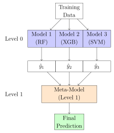
13.2 Blending

Definition 13.3 (Blending). Simplified version of stacking:

1. Split data: training set + hold-out validation set

2. Train base models on training set only

3. Generate predictions on hold-out set

4. Train meta-model on hold-out predictions

Difference from stacking: Uses single hold-out set instead of cross-validation.

Blending vs Stacking:

• Blending: Simpler, faster, but wastes data (hold-out not used for base model training)

• Stacking: More complex, uses all data efficiently, more robust

13.3 Choosing Base Models

Key Idea

Diversity is key! Choose base models that make different types of errors.

Good base model combinations:

• Different algorithms: Linear models, tree-based, neural networks, SVMs

• Different feature sets: Some models with all features, some with subsets

• Different hyperparameters: Multiple trees with different depths

• Different preprocessing: Some with PCA, some without; different scalings

Poor combination: 5 XGBoost models with similar hyperparameters (too correlated).

Meta-model choices:

• Linear/Logistic Regression: Simple, interpretable weights show model contributions

• Shallow tree: Can capture interactions between base models

• Neural network: Can learn complex combinations

Usually simple meta-models work best—base models already do the heavy lifting.

13.4 Practical Implementation

Implementation Notes

Stacking in Practice:

from sklearn.ensemble import StackingClassifier
from sklearn.linear_model import LogisticRegression
from sklearn.ensemble import RandomForestClassifier
from xgboost import XGBClassifier
from sklearn.svm import SVC

# Define base models
base_models = [
    ('rf', RandomForestClassifier(n_estimators=100)),
    ('xgb', XGBClassifier(n_estimators=100)),
    ('svm', SVC(probability=True))
]

# Define meta-model
meta_model = LogisticRegression()

# Create stacking ensemble
stacking = StackingClassifier(
    estimators=base_models,
    final_estimator=meta_model,
    cv=5  # 5-fold CV for out-of-fold predictions
)

# Train
stacking.fit(X_train, y_train)

# Predict
y_pred = stacking.predict(X_test)

Tips:

• Use 5-10 fold CV for stacking

• Include original features as inputs to meta-model (optional, often helps)

• For competitions: Stack multiple levels (3-4 levels possible)

• Ensure no information leakage between levels

• Validate on completely separate test set

13.5 Multi-Level Stacking

Definition 13.4 (Multi-Level Stacking). Extend to more than 2 levels:

• Level 0: Many diverse base models

• Level 1: Mid-level models on level-0 predictions

• Level 2: Top-level meta-model on level-1 predictions

• ... (can continue)

Caution: Diminishing returns after 2-3 levels. More levels increase:

• Complexity and computational cost

• Risk of overfitting

• Difficulty in debugging

Used mainly in competitions where every 0.01% matters.

13.6 Summary of Part 3

1. Ensemble Learning: Combine multiple models for better performance. Three paradigms: bagging, boosting, stacking.

2. Bagging/Random Forests: Train models independently on bootstrap samples. Reduces variance. RF adds feature randomness. OOB error provides free validation. Excellent general-purpose algorithm.

3. AdaBoost: Sequential training with adaptive example weights. Focuses on hard examples. Requires weak learners better than random.

4. Gradient Boosting: Generalizes boosting to arbitrary losses via functional gradient descent. XGBoost, LightGBM, CatBoost are modern optimized implementations with regularization.

5. Boosting Regularization: Learning rate, early stopping, subsampling, tree constraints. Essential to prevent overfitting.

6. Stacking: Train meta-model to combine base model predictions. Use CV to generate out-of-fold predictions. Learns optimal combination weights.

7. Model Selection: Random Forest for robust baseline. XGBoost/LightGBM for maximum accuracy (with tuning). Stacking to combine diverse models.

Next Steps: Part 4 covers neural networks and deep learning: perceptrons, backpropagation, CNNs, RNNs, Transformers, and modern optimization techniques.

Exercise 13.5.

1. Show that the probability of a specific example appearing in a bootstrap sample approaches \(1 - e^{-1} \approx 0.632\) as \(n \to \infty\).

2. For a Random Forest with 100 trees, each with 90% accuracy but only 50% correlated predictions, compute the expected ensemble accuracy if we use majority voting.

3. In AdaBoost, suppose a weak learner has error rate \(\epsilon_t = 0.4\). Compute its weight \(\alpha_t\). What happens if \(\epsilon_t = 0.5\) (random guessing)?

4. Explain why Gradient Boosting with squared loss is equivalent to sequentially fitting residuals.

5. Design a stacking ensemble with 4 base models for a classification task. What would you choose as base models and meta-model? Justify your choices.

6. Compare computational complexity: training 100 decision trees in Random Forest vs XGBoost. Which is faster and why?

7. For XGBoost, if learning rate is 0.01, how many trees would you typically need? What if learning rate is 0.3?

Part 4: Neural Networks and Deep Learning

14 The Perceptron

14.1 The Perceptron Model

Definition 14.1 (Perceptron). The perceptron is the simplest neural network unit, proposed by Rosenblatt (1958). For binary classification with \(y \in \{-1, +1\}\): \[\hat{y} = \text{sign}(\boldsymbol{w}^\top\boldsymbol{x} + b) = \text{sign}\left(\sum_{i=1}^d w_i x_i + b\right)\] where \(\boldsymbol{w}\) are weights, \(b\) is bias, and \(\text{sign}(z) = \begin{cases} +1 & z \geq 0 \\ -1 & z < 0 \end{cases}\).

Intuition 153. The perceptron is a linear classifier: it separates data with a hyperplane. Think of it as a simplified neuron that “fires” (+1) when the weighted input exceeds a threshold, and doesn’t fire (-1) otherwise.

Perceptron architecture: inputs, weights, sum, and sign activation

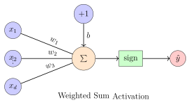
14.2 Perceptron Learning Algorithm

Algorithm Summary

Perceptron Learning Rule

Input: Training data \(\{(\boldsymbol{x}_i, y_i)\}_{i=1}^n\) with \(y_i \in \{-1, +1\}\)

Initialize: \(\boldsymbol{w} = \boldsymbol{0}\), \(b = 0\)

Repeat until convergence (or max iterations):

1. For each training example \((\boldsymbol{x}_i, y_i)\):

   • Compute prediction: \(\hat{y}_i = \text{sign}(\boldsymbol{w}^\top\boldsymbol{x}_i + b)\)

   • If \(\hat{y}_i \neq y_i\) (misclassified): \[\boldsymbol{w} \leftarrow \boldsymbol{w} + y_i\boldsymbol{x}_i, \quad b \leftarrow b + y_i\]

Output: Learned weights \(\boldsymbol{w}\) and bias \(b\)

Intuition 154. The update rule is intuitive:

• If true label is \(+1\) but we predicted \(-1\): increase \(\boldsymbol{w}\) in direction of \(\boldsymbol{x}\)

• If true label is \(-1\) but we predicted \(+1\): decrease \(\boldsymbol{w}\) in direction of \(\boldsymbol{x}\)

• Correct predictions: no update

This gradually rotates the hyperplane to correctly classify examples.

Theorem 14.4 (Perceptron Convergence Theorem). If the training data is linearly separable, the perceptron learning algorithm converges in a finite number of steps. Specifically, if all examples satisfy \(\left\lVert\boldsymbol{x}_i\right\rVert \leq R\) and there exists a unit vector \(\boldsymbol{w}^*\) with margin \(\gamma\) such that \(y_i(\boldsymbol{w}^{*\top}\boldsymbol{x}_i) \geq \gamma\) for all \(i\), then the algorithm makes at most \((R/\gamma)^2\) mistakes.

Sketch. Define mistake counter \(k\). After \(k\) mistakes, the weight vector is a sum of misclassified examples. Using properties of inner products and norms, one can show:

• Lower bound: \(\boldsymbol{w}_k \cdot \boldsymbol{w}^* \geq k\gamma\) (progress toward optimal)

• Upper bound: \(\left\lVert\boldsymbol{w}_k\right\rVert^2 \leq kR^2\) (bounded growth)

Combining via Cauchy-Schwarz: \(k \leq (R/\gamma)^2\). ◻

14.3 Limitations of the Perceptron

Key Idea

The XOR Problem:

Perceptron can only learn linearly separable functions. The XOR function is not linearly separable:

\(x_1\)	\(x_2\)	XOR
0	0	0
0	1	1
1	0	1
1	1	0

No single line can separate the 1s from the 0s!

XOR is not linearly separable

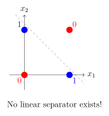
Solution: Use multiple perceptrons in layers \(\to\) Multi-Layer Perceptron (MLP) can learn XOR.

Historical note: This limitation caused the first “AI winter” in the 1970s. Minsky and Papert’s book (1969) highlighted these limitations, dampening enthusiasm until backpropagation was rediscovered in the 1980s.

15 Artificial Neural Networks

15.1 The Neuron Model

Definition 15.1 (Artificial Neuron). A neuron computes: \[a = f\left(\sum_{i=1}^d w_i x_i + b\right) = f(\boldsymbol{w}^\top\boldsymbol{x} + b)\] where:

• \(\boldsymbol{x} = [x_1, \ldots, x_d]^\top\) are inputs

• \(\boldsymbol{w} = [w_1, \ldots, w_d]^\top\) are weights

• \(b\) is bias

• \(f\) is the activation function

• \(a\) is the neuron’s output (activation)

15.2 Activation Functions

Definition 15.2 (Common Activation Functions). 1. Sigmoid: \[\sigma(z) = \frac{1}{1 + e^{-z}}, \quad \sigma'(z) = \sigma(z)(1-\sigma(z))\] Range: \((0, 1)\). Used in output layer for binary classification.

2. Hyperbolic Tangent (Tanh): \[\tanh(z) = \frac{e^z - e^{-z}}{e^z + e^{-z}}, \quad \tanh'(z) = 1 - \tanh^2(z)\] Range: \((-1, 1)\). Zero-centered (better than sigmoid for hidden layers).

3. ReLU (Rectified Linear Unit): \[\text{ReLU}(z) = \max(0, z), \quad \text{ReLU}'(z) = \begin{cases} 1 & z > 0 \\ 0 & z \leq 0 \end{cases}\] Most popular for hidden layers. Fast, addresses vanishing gradient.

4. Leaky ReLU: \[\text{LeakyReLU}(z) = \max(\alpha z, z), \quad \alpha \in (0, 1) \text{ typically } 0.01\] Prevents “dead neurons” (neurons that never activate).

5. GELU (Gaussian Error Linear Unit): \[\text{GELU}(z) = z \cdot \Phi(z)\] where \(\Phi\) is the Gaussian CDF. Smooth, used in Transformers (BERT, GPT).

6. Softmax (for output layer, multi-class): \[\text{softmax}(\boldsymbol{z})_i = \frac{e^{z_i}}{\sum_{j=1}^K e^{z_j}}\] Converts logits to probability distribution.

Common activation functions

Key Idea

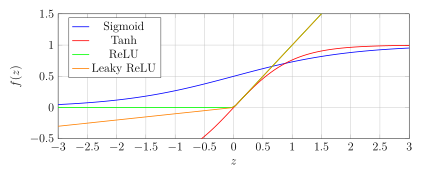
Why non-linear activations?

Without non-linearity, stacking layers is useless: \[f(\boldsymbol{W}_2 f(\boldsymbol{W}_1 \boldsymbol{x})) = f(\boldsymbol{W}_2 \boldsymbol{W}_1 \boldsymbol{x}) = f(\boldsymbol{W} \boldsymbol{x})\] Multiple linear layers collapse to a single linear transformation. Non-linear activations enable neural networks to approximate any continuous function (Universal Approximation Theorem).

Choosing activation:

• Hidden layers: ReLU (default), Leaky ReLU, GELU

• Output layer:

  • Binary classification: Sigmoid

  • Multi-class: Softmax

  • Regression: Linear (no activation)

15.3 Multi-Layer Perceptron (MLP)

Definition 15.3 (Feedforward Neural Network). An MLP with \(L\) layers has:

• Input layer: \(\boldsymbol{x} = \boldsymbol{a}^{(0)} \in \mathbb{R}^{d_0}\)

• Hidden layers \(\ell = 1, \ldots, L-1\): \[\boldsymbol{z}^{(\ell)} = \boldsymbol{W}^{(\ell)}\boldsymbol{a}^{(\ell-1)} + \boldsymbol{b}^{(\ell)}, \quad \boldsymbol{a}^{(\ell)} = f^{(\ell)}(\boldsymbol{z}^{(\ell)})\]

• Output layer \(\ell = L\): \[\boldsymbol{z}^{(L)} = \boldsymbol{W}^{(L)}\boldsymbol{a}^{(L-1)} + \boldsymbol{b}^{(L)}, \quad \hat{\boldsymbol{y}} = \boldsymbol{a}^{(L)} = f^{(L)}(\boldsymbol{z}^{(L)})\]

where \(\boldsymbol{W}^{(\ell)} \in \mathbb{R}^{d_\ell \times d_{\ell-1}}\), \(\boldsymbol{b}^{(\ell)} \in \mathbb{R}^{d_\ell}\).

Multi-Layer Perceptron with 2 hidden layers

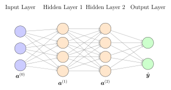
15.4 Forward Propagation

Algorithm Summary

Forward Propagation Algorithm

Input: Example \(\boldsymbol{x}\), network parameters \(\{\boldsymbol{W}^{(\ell)}, \boldsymbol{b}^{(\ell)}\}_{\ell=1}^L\)

Initialize: \(\boldsymbol{a}^{(0)} = \boldsymbol{x}\)

For \(\ell = 1\) to \(L\):

1. Compute pre-activation: \(\boldsymbol{z}^{(\ell)} = \boldsymbol{W}^{(\ell)}\boldsymbol{a}^{(\ell-1)} + \boldsymbol{b}^{(\ell)}\)

2. Compute activation: \(\boldsymbol{a}^{(\ell)} = f^{(\ell)}(\boldsymbol{z}^{(\ell)})\)

Output: Prediction \(\hat{\boldsymbol{y}} = \boldsymbol{a}^{(L)}\)

15.5 Loss Functions

Definition 15.4 (Common Loss Functions). Regression (continuous output):

• Mean Squared Error: \(\mathcal{L}= \frac{1}{n}\sum_{i=1}^n \left\lVert\boldsymbol{y}_i - \hat{\boldsymbol{y}}_i\right\rVert_2^2\)

• Mean Absolute Error: \(\mathcal{L}= \frac{1}{n}\sum_{i=1}^n \left\lVert\boldsymbol{y}_i - \hat{\boldsymbol{y}}_i\right\rVert_1\)

Binary Classification:

• Binary Cross-Entropy: \[\mathcal{L}= -\frac{1}{n}\sum_{i=1}^n [y_i\log(\hat{y}_i) + (1-y_i)\log(1-\hat{y}_i)]\]

Multi-Class Classification:

• Categorical Cross-Entropy: \[\mathcal{L}= -\frac{1}{n}\sum_{i=1}^n \sum_{k=1}^K y_{ik}\log(\hat{y}_{ik})\] where \(\boldsymbol{y}_i\) is one-hot encoded.

15.6 Backpropagation

Backpropagation efficiently computes gradients using the chain rule.

Theorem 15.5 (Backpropagation Algorithm). For a network with \(L\) layers, we compute gradients backward from output to input.

Output layer gradient: \[\boldsymbol{\delta}^{(L)} = \nabla_{\boldsymbol{a}^{(L)}} \mathcal{L}\odot f'^{(L)}(\boldsymbol{z}^{(L)})\] where \(\odot\) is element-wise product.

Hidden layer gradients (for \(\ell = L-1, L-2, \ldots, 1\)): \[\boldsymbol{\delta}^{(\ell)} = (\boldsymbol{W}^{(\ell+1)})^\top \boldsymbol{\delta}^{(\ell+1)} \odot f'^{(\ell)}(\boldsymbol{z}^{(\ell)})\]

Parameter gradients: \[\nabla_{\boldsymbol{W}^{(\ell)}} \mathcal{L}= \boldsymbol{\delta}^{(\ell)} (\boldsymbol{a}^{(\ell-1)})^\top, \quad \nabla_{\boldsymbol{b}^{(\ell)}} \mathcal{L}= \boldsymbol{\delta}^{(\ell)}\]

Derivation Sketch. By chain rule, for layer \(\ell\): \[\frac{\partial \mathcal{L}}{\partial \boldsymbol{W}^{(\ell)}} = \frac{\partial \mathcal{L}}{\partial \boldsymbol{z}^{(\ell)}} \cdot \frac{\partial \boldsymbol{z}^{(\ell)}}{\partial \boldsymbol{W}^{(\ell)}}\] Define \(\boldsymbol{\delta}^{(\ell)} = \frac{\partial \mathcal{L}}{\partial \boldsymbol{z}^{(\ell)}}\) (the “error” at layer \(\ell\)).

For the output layer: \[\boldsymbol{\delta}^{(L)} = \frac{\partial \mathcal{L}}{\partial \boldsymbol{a}^{(L)}} \cdot \frac{\partial \boldsymbol{a}^{(L)}}{\partial \boldsymbol{z}^{(L)}} = \nabla_{\boldsymbol{a}^{(L)}} \mathcal{L}\odot f'^{(L)}(\boldsymbol{z}^{(L)})\]

For hidden layers, using chain rule through layer \(\ell+1\): \[\boldsymbol{\delta}^{(\ell)} = \frac{\partial \boldsymbol{z}^{(\ell+1)}}{\partial \boldsymbol{a}^{(\ell)}} \cdot \frac{\partial \mathcal{L}}{\partial \boldsymbol{z}^{(\ell+1)}} \cdot \frac{\partial \boldsymbol{a}^{(\ell)}}{\partial \boldsymbol{z}^{(\ell)}} = (\boldsymbol{W}^{(\ell+1)})^\top \boldsymbol{\delta}^{(\ell+1)} \odot f'^{(\ell)}(\boldsymbol{z}^{(\ell)})\]

Finally: \[\nabla_{\boldsymbol{W}^{(\ell)}} \mathcal{L}= \boldsymbol{\delta}^{(\ell)} (\boldsymbol{a}^{(\ell-1)})^\top\] ◻

Algorithm Summary

Backpropagation Algorithm

Forward Pass: Compute all \(\boldsymbol{z}^{(\ell)}\) and \(\boldsymbol{a}^{(\ell)}\) for \(\ell = 1, \ldots, L\)

Backward Pass:

1. Compute output error: \(\boldsymbol{\delta}^{(L)} = \nabla_{\boldsymbol{a}^{(L)}} \mathcal{L}\odot f'^{(L)}(\boldsymbol{z}^{(L)})\)

2. For \(\ell = L-1\) down to \(1\):

   • Backpropagate error: \(\boldsymbol{\delta}^{(\ell)} = (\boldsymbol{W}^{(\ell+1)})^\top \boldsymbol{\delta}^{(\ell+1)} \odot f'^{(\ell)}(\boldsymbol{z}^{(\ell)})\)

   • Compute weight gradient: \(\nabla_{\boldsymbol{W}^{(\ell)}} \mathcal{L}= \boldsymbol{\delta}^{(\ell)} (\boldsymbol{a}^{(\ell-1)})^\top\)

   • Compute bias gradient: \(\nabla_{\boldsymbol{b}^{(\ell)}} \mathcal{L}= \boldsymbol{\delta}^{(\ell)}\)

Update: \(\boldsymbol{W}^{(\ell)} \leftarrow \boldsymbol{W}^{(\ell)} - \eta \nabla_{\boldsymbol{W}^{(\ell)}} \mathcal{L}\) for all layers

Key Idea

Why backpropagation is efficient:

Naive approach: Compute each partial derivative independently \(\to\) \(O(n \cdot p)\) where \(p\) is number of parameters.

Backpropagation: Compute all gradients in one backward pass \(\to\) \(O(p)\), roughly the same as one forward pass.

The key insight: Reuse intermediate computations. The error \(\boldsymbol{\delta}^{(\ell)}\) at layer \(\ell\) depends on \(\boldsymbol{\delta}^{(\ell+1)}\), so we propagate errors backward efficiently.

15.7 Vanishing and Exploding Gradients

Definition 15.6 (Gradient Vanishing). In deep networks with sigmoid/tanh activations, gradients can become very small as they propagate backward, making early layers learn very slowly.

Why? \(\sigma'(z) = \sigma(z)(1-\sigma(z)) \leq 0.25\). For a network with \(L\) layers: \[\frac{\partial \mathcal{L}}{\partial \boldsymbol{W}^{(1)}} \propto \prod_{\ell=1}^L \sigma'(z^{(\ell)}) \boldsymbol{W}^{(\ell)}\] If \(\sigma'(z) \approx 0.1\), then gradient \(\approx 0.1^L \to 0\) exponentially fast.

Definition 15.7 (Gradient Exploding). Conversely, if weights are large or activations unbounded, gradients can explode: \[\text{gradient} \propto \prod_{\ell} \boldsymbol{W}^{(\ell)} \to \infty\] Causes numerical instability, NaN values.

Key Idea

Solutions to Vanishing/Exploding Gradients:

1. Better Activation Functions:

• ReLU: \(f'(z) = 1\) for \(z > 0\) (no vanishing in positive region)

• Leaky ReLU, ELU: Address “dying ReLU” problem

2. Careful Weight Initialization:

• Xavier/Glorot: \(\boldsymbol{W} \sim \mathcal{N}(0, 2/(d_{\text{in}} + d_{\text{out}}))\)

• He initialization (for ReLU): \(\boldsymbol{W} \sim \mathcal{N}(0, 2/d_{\text{in}})\)

3. Batch Normalization: Normalize activations at each layer

4. Residual Connections (ResNet): Skip connections allow gradients to flow directly

5. Gradient Clipping: Cap gradients at a maximum value (for exploding)

6. LSTM/GRU: Specifically designed for RNNs to address vanishing gradients

16 Optimization in Deep Learning

16.1 Stochastic Gradient Descent Variants

16.1.1 Momentum

Definition 16.1 (SGD with Momentum). Accumulate past gradients to accelerate convergence: \[\boldsymbol{v}_t = \beta \boldsymbol{v}_{t-1} + \eta \nabla_{\boldsymbol{w}} \mathcal{L}, \quad \boldsymbol{w}_{t+1} = \boldsymbol{w}_t - \boldsymbol{v}_t\] Typical: \(\beta = 0.9\). Alternatively, some formulations use \(\boldsymbol{v}_t = \beta \boldsymbol{v}_{t-1} + \nabla_{\boldsymbol{w}} \mathcal{L}\) with \(\boldsymbol{w}_{t+1} = \boldsymbol{w}_t - \eta \boldsymbol{v}_t\).

Intuition 164. Momentum accelerates in directions with consistent gradients and dampens oscillations. Think of a ball rolling down a hill—it builds up speed in the downhill direction.

16.1.2 RMSProp

Definition 16.3 (RMSProp (Root Mean Square Propagation)). Adapt learning rate per parameter using moving average of squared gradients: \[\boldsymbol{s}_t = \beta \boldsymbol{s}_{t-1} + (1-\beta)(\nabla_{\boldsymbol{w}} \mathcal{L})^2, \quad \boldsymbol{w}_{t+1} = \boldsymbol{w}_t - \frac{\eta}{\sqrt{\boldsymbol{s}_t + \epsilon}} \odot \nabla_{\boldsymbol{w}} \mathcal{L}\] Typical: \(\beta = 0.9\), \(\epsilon = 10^{-8}\).

Intuition 166. RMSProp divides the learning rate by a running average of the gradient magnitude. Parameters with large gradients get smaller effective learning rates; parameters with small gradients get larger effective rates. This helps with different scales across parameters.

16.1.3 Adam

Definition 16.5 (Adam (Adaptive Moment Estimation)). Combines momentum and RMSProp: \[\begin{align} \boldsymbol{m}_t &= \beta_1 \boldsymbol{m}_{t-1} + (1-\beta_1)\nabla_{\boldsymbol{w}} \mathcal{L}&& \text{(first moment)} \\ \boldsymbol{v}_t &= \beta_2 \boldsymbol{v}_{t-1} + (1-\beta_2)(\nabla_{\boldsymbol{w}} \mathcal{L})^2 && \text{(second moment)} \\ \hat{\boldsymbol{m}}_t &= \frac{\boldsymbol{m}_t}{1 - \beta_1^t}, \quad \hat{\boldsymbol{v}}_t = \frac{\boldsymbol{v}_t}{1 - \beta_2^t} && \text{(bias correction)} \\ \boldsymbol{w}_{t+1} &= \boldsymbol{w}_t - \frac{\eta}{\sqrt{\hat{\boldsymbol{v}}_t} + \epsilon} \odot \hat{\boldsymbol{m}}_t \end{align}\] Typical: \(\beta_1 = 0.9\), \(\beta_2 = 0.999\), \(\eta = 0.001\), \(\epsilon = 10^{-8}\).

Key Idea

Adam is the default optimizer for deep learning:

• Combines benefits of momentum (acceleration) and RMSProp (adaptive rates)

• Works well across a wide range of problems

• Bias correction ensures good estimates early in training

• Relatively insensitive to hyperparameters

Variants:

• AdamW: Adam with decoupled weight decay (better regularization)

• AMSGrad: Fixes potential convergence issues in Adam

• Nadam: Nesterov + Adam

16.2 Learning Rate Schedules

Definition 16.6 (Learning Rate Decay Strategies). 1. Step Decay: \[\eta_t = \eta_0 \cdot \gamma^{\lfloor t / k \rfloor}\] Drop learning rate by factor \(\gamma\) every \(k\) epochs.

2. Exponential Decay: \[\eta_t = \eta_0 e^{-\lambda t}\]

3. Cosine Annealing: \[\eta_t = \eta_{\min} + \frac{1}{2}(\eta_{\max} - \eta_{\min})\left(1 + \cos\left(\frac{t}{T}\pi\right)\right)\] Smoothly decreases from \(\eta_{\max}\) to \(\eta_{\min}\) over \(T\) steps.

4. Warm-up + Decay:

• Linearly increase LR from 0 to \(\eta_0\) over first few epochs (warm-up)

• Then apply decay schedule

Used in Transformers.

16.3 Batch Normalization

Definition 16.7 (Batch Normalization). For a mini-batch \(\mathcal{B} = \{\boldsymbol{x}_1, \ldots, \boldsymbol{x}_m\}\), normalize each feature: \[\begin{align} \mu_{\mathcal{B}} &= \frac{1}{m}\sum_{i=1}^m x_i \\ \sigma_{\mathcal{B}}^2 &= \frac{1}{m}\sum_{i=1}^m (x_i - \mu_{\mathcal{B}})^2 \\ \hat{x}_i &= \frac{x_i - \mu_{\mathcal{B}}}{\sqrt{\sigma_{\mathcal{B}}^2 + \epsilon}} \\ y_i &= \gamma \hat{x}_i + \beta \end{align}\] where \(\gamma\) and \(\beta\) are learnable parameters (scale and shift).

Key Idea

Benefits of Batch Normalization:

• Faster training: Can use higher learning rates

• Reduces internal covariate shift: Stabilizes distribution of layer inputs

• Regularization effect: Adds noise (batch statistics), reduces overfitting

• Less sensitive to initialization: Makes training more robust

Where to apply: After linear transformation, before activation: \[\boldsymbol{z} = \boldsymbol{W}\boldsymbol{a}^{(\ell-1)} + \boldsymbol{b} \to \text{BatchNorm}(\boldsymbol{z}) \to f(\cdot)\]

At test time: Use running averages of \(\mu\) and \(\sigma^2\) computed during training (no batch available).

16.4 Dropout

Definition 16.8 (Dropout). During training, randomly set activations to zero with probability \(p\) (typically 0.5): \[\tilde{a}_i = \begin{cases} 0 & \text{with probability } p \\ a_i / (1-p) & \text{with probability } 1-p \end{cases}\] At test time, use all neurons (no dropout).

Intuition 171. Dropout prevents co-adaptation of neurons. By randomly dropping neurons, the network cannot rely on any specific neurons, forcing it to learn robust features. It’s like training an ensemble of networks that share weights.

Key Idea

Dropout as Regularization:

• Prevents overfitting, especially in fully-connected layers

• Typical \(p\): 0.2-0.5 for hidden layers, 0-0.2 for input layer

• Not typically used in convolutional layers (they have fewer parameters)

• Can be viewed as approximate Bayesian inference

Variants:

• DropConnect: Drop weights instead of activations

• Spatial Dropout: For CNNs, drop entire feature maps

17 Deep Architectures

17.1 Convolutional Neural Networks (CNNs)

17.1.1 Motivation for CNNs

Problem with fully-connected networks for images:

• Image \(32 \times 32 \times 3\) has 3072 pixels. Hidden layer with 1000 neurons \(\to\) 3M parameters just in first layer!

• No spatial structure: treats pixels far apart the same as nearby pixels

• Not translation invariant: must learn same feature at every location

CNNs exploit:

• Local connectivity: Neurons connect to small spatial regions

• Weight sharing: Same filter applied across entire image

• Translation equivariance: Features detected anywhere in the image

17.1.2 Convolutional Layer

Definition 17.1 (Convolution Operation). For input \(\boldsymbol{X} \in \mathbb{R}^{H \times W \times C}\) and filter \(\boldsymbol{K} \in \mathbb{R}^{F \times F \times C}\): \[Y[i,j] = \sum_{di=0}^{F-1}\sum_{dj=0}^{F-1}\sum_{c=1}^C X[i+di, j+dj, c] \cdot K[di, dj, c] + b\] Apply this for all positions \((i,j)\) to get feature map \(\boldsymbol{Y}\).

With \(D\) filters, output has shape \((H', W', D)\) where: \[H' = \frac{H - F + 2P}{S} + 1, \quad W' = \frac{W - F + 2P}{S} + 1\] \(P\) = padding, \(S\) = stride.

Convolution operation: filter slides across input to produce output feature map

Key Idea

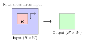
Key Concepts:

1. Receptive Field: Region of input that affects one output neuron. Deeper layers have larger receptive fields.

2. Padding:

• Valid (no padding): Output size decreases

• Same (pad to maintain size): \(P = (F-1)/2\) for stride 1

3. Stride: Step size. Larger stride \(\to\) smaller output, reduces computation.

4. Number of Parameters: For filter \(F \times F \times C\) with \(D\) filters: \[\text{params} = (F \times F \times C + 1) \times D\] Much smaller than fully-connected layer!

17.1.3 Pooling Layers

Definition 17.2 (Pooling). Downsampling operation to reduce spatial dimensions:

Max Pooling: Take maximum in each region \[Y[i,j] = \max_{di,dj} X[i \cdot S + di, j \cdot S + dj]\]

Average Pooling: Take average \[Y[i,j] = \frac{1}{F^2}\sum_{di,dj} X[i \cdot S + di, j \cdot S + dj]\]

Common: \(2 \times 2\) pooling with stride 2 (halves dimensions).

Benefits of pooling:

• Reduces computation and memory

• Provides translation invariance

• Increases receptive field

17.1.4 Common CNN Architectures

Example 17.3 (LeNet-5 (1998) - Digit Recognition). Input (32×32) → Conv(6 filters, 5×5) → Pool(2×2) → Conv(16 filters, 5×5) → Pool(2×2) → FC(120) → FC(84) → FC(10)

First successful CNN, used for ZIP code recognition.

Example 17.4 (AlexNet (2012) - ImageNet Winner).

• 8 layers (5 conv, 3 FC)

• ReLU activation (first major use)

• Dropout for regularization

• Data augmentation

• 60M parameters, reduced top-5 error from 26% to 15.3%

Marked the beginning of the deep learning revolution.

Example 17.5 (VGGNet (2014)).

• Very deep (16-19 layers)

• Only \(3 \times 3\) convolutions (smaller filters, stacked)

• Showed depth is crucial

• 138M parameters (VGG-16)

Example 17.6 (ResNet (2015) - 152 Layers). Key innovation: Residual Connections

Instead of learning \(\mathcal{H}(\boldsymbol{x})\), learn residual \(\mathcal{F}(\boldsymbol{x})\) where: \[\mathcal{H}(\boldsymbol{x}) = \mathcal{F}(\boldsymbol{x}) + \boldsymbol{x}\] Skip connections allow gradients to flow directly, enabling very deep networks.

Won ImageNet 2015, error rate 3.6% (below human performance!).

ResNet residual block with skip connection

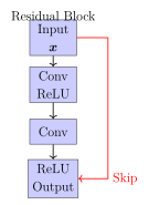
17.2 Recurrent Neural Networks (RNNs)

17.2.1 Sequence Modeling

Motivation: Many problems involve sequences:

• Text: “The cat sat on the ___” (predict next word)

• Time series: Stock prices, weather data

• Speech: Audio to text

• Video: Frame-by-frame analysis

Challenge: Variable-length inputs and dependencies between timesteps.

17.2.2 Vanilla RNN

Definition 17.7 (Recurrent Neural Network). At timestep \(t\): \[\begin{align} \boldsymbol{h}_t &= f(\boldsymbol{W}_{hh}\boldsymbol{h}_{t-1} + \boldsymbol{W}_{xh}\boldsymbol{x}_t + \boldsymbol{b}_h) \\ \boldsymbol{y}_t &= \boldsymbol{W}_{hy}\boldsymbol{h}_t + \boldsymbol{b}_y \end{align}\] where:

• \(\boldsymbol{x}_t\): input at time \(t\)

• \(\boldsymbol{h}_t\): hidden state (memory)

• \(\boldsymbol{y}_t\): output at time \(t\)

• \(f\): activation (typically tanh or ReLU)

RNN unrolled through time. Red arrows show recurrent connections.

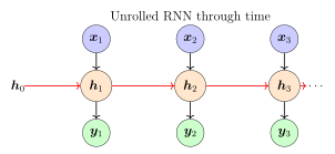
17.2.3 Backpropagation Through Time (BPTT)

Training RNNs: Unfold network through time and apply backpropagation. Gradients flow backward through all timesteps.

Problem: Vanishing gradients are even worse in RNNs! \[\frac{\partial \mathcal{L}}{\partial \boldsymbol{h}_1} \propto \prod_{t=2}^T \frac{\partial \boldsymbol{h}_t}{\partial \boldsymbol{h}_{t-1}} = \prod_{t=2}^T \boldsymbol{W}_{hh} \cdot f'(\boldsymbol{z}_t)\] For long sequences (\(T\) large), gradient vanishes or explodes exponentially.

17.2.4 LSTM (Long Short-Term Memory)

Definition 17.8 (LSTM Cell). LSTM uses gates to control information flow:

Forget gate: What to forget from cell state \[\boldsymbol{f}_t = \sigma(\boldsymbol{W}_f[\boldsymbol{h}_{t-1}, \boldsymbol{x}_t] + \boldsymbol{b}_f)\]

Input gate: What new information to add \[\boldsymbol{i}_t = \sigma(\boldsymbol{W}_i[\boldsymbol{h}_{t-1}, \boldsymbol{x}_t] + \boldsymbol{b}_i)\] \[\tilde{\boldsymbol{c}}_t = \tanh(\boldsymbol{W}_c[\boldsymbol{h}_{t-1}, \boldsymbol{x}_t] + \boldsymbol{b}_c)\]

Cell state update: \[\boldsymbol{c}_t = \boldsymbol{f}_t \odot \boldsymbol{c}_{t-1} + \boldsymbol{i}_t \odot \tilde{\boldsymbol{c}}_t\]

Output gate: What to output \[\boldsymbol{o}_t = \sigma(\boldsymbol{W}_o[\boldsymbol{h}_{t-1}, \boldsymbol{x}_t] + \boldsymbol{b}_o)\] \[\boldsymbol{h}_t = \boldsymbol{o}_t \odot \tanh(\boldsymbol{c}_t)\]

Key Idea

Why LSTM works:

• Cell state \(\boldsymbol{c}_t\) acts as a “conveyor belt” for information

• Gates (sigmoid \(\in [0,1]\)) control what flows through

• Forget gate can preserve gradients over long sequences

• Addresses vanishing gradient problem

When to use LSTM:

• Long sequences (>50-100 timesteps)

• Long-term dependencies matter

• Text generation, machine translation, speech recognition

17.2.5 GRU (Gated Recurrent Unit)

Definition 17.9 (GRU). Simplified version of LSTM with fewer parameters:

Update gate: \[\boldsymbol{z}_t = \sigma(\boldsymbol{W}_z[\boldsymbol{h}_{t-1}, \boldsymbol{x}_t])\]

Reset gate: \[\boldsymbol{r}_t = \sigma(\boldsymbol{W}_r[\boldsymbol{h}_{t-1}, \boldsymbol{x}_t])\]

Candidate hidden state: \[\tilde{\boldsymbol{h}}_t = \tanh(\boldsymbol{W}[\boldsymbol{r}_t \odot \boldsymbol{h}_{t-1}, \boldsymbol{x}_t])\]

Hidden state update: \[\boldsymbol{h}_t = (1 - \boldsymbol{z}_t) \odot \boldsymbol{h}_{t-1} + \boldsymbol{z}_t \odot \tilde{\boldsymbol{h}}_t\]

GRU vs LSTM:

• GRU: Simpler, fewer parameters, faster training

• LSTM: More expressive, better for very long sequences

• Performance often similar—try both!

17.3 Transformers and Attention

17.3.1 Limitations of RNNs

• Sequential computation: Cannot parallelize (must process \(t-1\) before \(t\))

• Long-range dependencies: Still struggle despite LSTM/GRU

• Fixed hidden state: Must compress entire history into \(\boldsymbol{h}_t\)

Solution: Attention mechanism—directly access any part of the input.

17.3.2 Attention Mechanism

Definition 17.10 (Attention). Given query \(\boldsymbol{q}\), keys \(\boldsymbol{K} = [\boldsymbol{k}_1, \ldots, \boldsymbol{k}_n]\), and values \(\boldsymbol{V} = [\boldsymbol{v}_1, \ldots, \boldsymbol{v}_n]\):

1. Compute attention scores: \[e_i = \text{score}(\boldsymbol{q}, \boldsymbol{k}_i)\] Common: \(\text{score}(\boldsymbol{q}, \boldsymbol{k}) = \boldsymbol{q}^\top\boldsymbol{k}\) (dot product)

2. Normalize to get attention weights: \[\alpha_i = \frac{\exp(e_i)}{\sum_j \exp(e_j)} \quad \text{(softmax)}\]

3. Compute weighted sum: \[\text{context} = \sum_{i=1}^n \alpha_i \boldsymbol{v}_i\]

Intuition 182. Attention allows the model to “focus” on relevant parts of the input. For translation, when generating word \(t\), attention looks at all source words and focuses on the most relevant ones.

17.3.3 Scaled Dot-Product Attention

Definition 17.12 (Scaled Dot-Product Attention). \[\text{Attention}(\boldsymbol{Q}, \boldsymbol{K}, \boldsymbol{V}) = \text{softmax}\left(\frac{\boldsymbol{Q}\boldsymbol{K}^\top}{\sqrt{d_k}}\right)\boldsymbol{V}\] where \(\boldsymbol{Q} \in \mathbb{R}^{n \times d_k}\), \(\boldsymbol{K} \in \mathbb{R}^{m \times d_k}\), \(\boldsymbol{V} \in \mathbb{R}^{m \times d_v}\).

Scaling by \(\sqrt{d_k}\) prevents softmax saturation for large \(d_k\).

17.3.4 Transformer Architecture

Definition 17.13 (Transformer (Vaswani et al., 2017)). Uses only attention mechanisms (no recurrence):

Key components:

1. Multi-Head Attention: Multiple attention operations in parallel \[\text{MultiHead}(\boldsymbol{Q}, \boldsymbol{K}, \boldsymbol{V}) = \text{Concat}(\text{head}_1, \ldots, \text{head}_h)\boldsymbol{W}^O\] where \(\text{head}_i = \text{Attention}(\boldsymbol{Q}\boldsymbol{W}_i^Q, \boldsymbol{K}\boldsymbol{W}_i^K, \boldsymbol{V}\boldsymbol{W}_i^V)\)

2. Positional Encoding: Add position information (since no recurrence) \[PE_{(pos, 2i)} = \sin(pos/10000^{2i/d}), \quad PE_{(pos, 2i+1)} = \cos(pos/10000^{2i/d})\]

3. Feed-Forward Networks: Applied position-wise \[\text{FFN}(\boldsymbol{x}) = \max(0, \boldsymbol{x}\boldsymbol{W}_1 + \boldsymbol{b}_1)\boldsymbol{W}_2 + \boldsymbol{b}_2\]

4. Layer Normalization and Residual Connections

Key Idea

Why Transformers Revolutionized NLP:

• Parallelization: All positions processed simultaneously

• Long-range dependencies: Direct connections between any positions

• Scalability: Can train on massive datasets efficiently

• Transfer learning: Pre-train on large corpus, fine-tune on task

Impact:

• BERT (2018): Bidirectional Transformer for language understanding

• GPT series (2018-2023): Decoder-only Transformers for generation

• Vision Transformers (ViT): Applied to images

• Now the dominant architecture in NLP and increasingly in vision

17.4 Summary of Part 4

1. Perceptron: First neural network model. Linear classifier with convergence guarantee for separable data. Cannot learn XOR (not linearly separable).

2. MLPs: Stack layers with non-linear activations. Universal approximators. Trained via backpropagation—efficient gradient computation using chain rule.

3. Activation Functions: ReLU is default for hidden layers (addresses vanishing gradients). Sigmoid/Softmax for output. GELU in modern architectures.

4. Optimization: Adam is standard optimizer. Learning rate schedules improve convergence. Batch normalization and dropout for regularization.

5. CNNs: Exploit spatial structure via convolution and pooling. Weight sharing reduces parameters. ResNet’s skip connections enable very deep networks.

6. RNNs: Process sequences with recurrent connections. Vanilla RNNs suffer from vanishing gradients. LSTM/GRU use gates to maintain long-term memory.

7. Transformers: Attention mechanism allows direct access to all inputs. Fully parallelizable, handles long-range dependencies. Dominant architecture in modern NLP and increasingly in vision.

Next Steps: Part 5 explores unsupervised learning: clustering, dimensionality reduction, and methods for discovering structure without labels.

Exercise 17.14.

1. Prove that a single-layer perceptron cannot learn the XOR function. Show that a two-layer network with 2 hidden neurons can learn it.

2. Derive the backpropagation equations for a 3-layer network with sigmoid activations and MSE loss.

3. For a conv layer with input \(32 \times 32 \times 3\), filter size \(5 \times 5\), 64 filters, stride 1, padding 2: compute output dimensions and number of parameters.

4. Explain why ReLU helps with vanishing gradients compared to sigmoid. What is the “dying ReLU” problem?

5. Implement gradient descent with momentum by hand for \(f(x) = x^2\), starting from \(x_0 = 10\), with \(\eta = 0.1\), \(\beta = 0.9\). Show 5 iterations.

6. In an LSTM, what happens if the forget gate outputs all 1s? All 0s?

7. For scaled dot-product attention with \(d_k = 64\), why do we divide by \(\sqrt{64} = 8\)? What happens without scaling?

8. Compare computational complexity: training a 10-layer RNN vs a 10-layer Transformer on a sequence of length 100. Which is faster and why?

Part 5: Unsupervised Learning

18 Introduction to Unsupervised Learning

Definition 18.1 (Unsupervised Learning). In unsupervised learning, we have only input data \(\mathcal{D} = \{\boldsymbol{x}_1, \boldsymbol{x}_2, \ldots, \boldsymbol{x}_n\}\) without labels. The goal is to discover hidden structure or patterns in the data.

Key Idea

Main Tasks in Unsupervised Learning:

• Clustering: Group similar examples together

• Dimensionality Reduction: Find lower-dimensional representations

• Density Estimation: Model the probability distribution \(P(\boldsymbol{x})\)

• Anomaly Detection: Identify unusual or outlier examples

• Association Rules: Discover relationships between variables

Why Unsupervised Learning?

• Labeled data is expensive; unlabeled data is abundant

• Discover hidden structures humans might miss

• Preprocessing for supervised learning (feature extraction)

• Understand data distribution and relationships

19 Clustering

19.1 K-Means Clustering

19.1.1 Problem Formulation

Definition 19.1 (K-Means Objective). Given data \(\{\boldsymbol{x}_i\}_{i=1}^n\) and desired number of clusters \(K\), find:

• Cluster centers (centroids) \(\{\boldsymbol{\mu}_k\}_{k=1}^K\)

• Cluster assignments \(\{c_i\}_{i=1}^n\) where \(c_i \in \{1, \ldots, K\}\)

to minimize within-cluster sum of squares: \[J = \sum_{i=1}^n \left\lVert\boldsymbol{x}_i - \boldsymbol{\mu}_{c_i}\right\rVert_2^2 = \sum_{k=1}^K \sum_{i: c_i=k} \left\lVert\boldsymbol{x}_i - \boldsymbol{\mu}_k\right\rVert_2^2\]

Intuition 188. K-means finds \(K\) cluster centers and assigns each point to its nearest center. The objective minimizes the total distance from points to their assigned centers—we want tight, compact clusters.

19.1.2 Lloyd’s Algorithm

Algorithm Summary

K-Means Algorithm (Lloyd’s Algorithm)

Input: Data \(\{\boldsymbol{x}_i\}_{i=1}^n\), number of clusters \(K\), max iterations \(T\)

Initialize: Randomly select \(K\) points as initial centroids \(\{\boldsymbol{\mu}_k\}_{k=1}^K\)

Repeat until convergence (or \(T\) iterations):

1. Assignment step: Assign each point to nearest centroid \[c_i = \mathop{\mathrm{arg\,min}}_{k \in \{1,\ldots,K\}} \left\lVert\boldsymbol{x}_i - \boldsymbol{\mu}_k\right\rVert_2^2\]

2. Update step: Recompute centroids as mean of assigned points \[\boldsymbol{\mu}_k = \frac{1}{|C_k|}\sum_{i \in C_k} \boldsymbol{x}_i\] where \(C_k = \{i : c_i = k\}\) is the set of points assigned to cluster \(k\).

3. Check convergence: If assignments don’t change, stop

Output: Cluster centers \(\{\boldsymbol{\mu}_k\}\) and assignments \(\{c_i\}\)

Theorem 19.3 (K-Means Convergence). Lloyd’s algorithm is guaranteed to converge to a local minimum of \(J\). The objective decreases (or stays the same) at each iteration:

• Assignment step: Each point moves to nearest center \(\to\) \(J\) decreases

• Update step: Each center moves to mean of its cluster \(\to\) \(J\) decreases

Since \(J \geq 0\) and there are finitely many possible assignments, the algorithm must converge.

K-Means iterations: Initial random centroids converge to cluster centers

Key Idea

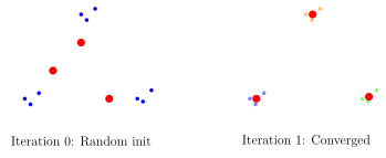
Initialization Matters!

K-means finds a local minimum, which depends on initialization.

K-Means++ Initialization:

1. Choose first center uniformly at random

2. For each subsequent center, choose point with probability proportional to squared distance from nearest existing center

3. Repeat until \(K\) centers chosen

This spreads out initial centers, leading to better final clusters.

Multiple Runs: Run K-means multiple times (10-100) with different initializations, keep the best result (lowest \(J\)).

19.1.3 Choosing K (Number of Clusters)

Definition 19.4 (Elbow Method). Plot \(J\) (within-cluster sum of squares) vs \(K\). Look for an “elbow”—a point where \(J\) stops decreasing rapidly.

Elbow method: \(J\) decreases rapidly until \(K=4\), then flattens

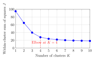
Definition 19.5 (Silhouette Score). For each point \(i\), compute:

• \(a_i\): Average distance to other points in same cluster

• \(b_i\): Average distance to points in nearest other cluster

Silhouette coefficient: \[s_i = \frac{b_i - a_i}{\max(a_i, b_i)} \in [-1, 1]\]

• \(s_i \approx 1\): Well clustered (far from other clusters)

• \(s_i \approx 0\): On boundary between clusters

• \(s_i < 0\): Possibly assigned to wrong cluster

Silhouette score: Average \(s_i\) over all points. Higher is better.

19.1.4 Advantages and Limitations

Key Idea

Advantages of K-Means:

• Simple, intuitive, easy to implement

• Fast: \(O(nKdT)\) where \(T\) is number of iterations (usually small)

• Scales to large datasets

• Works well for spherical, well-separated clusters

Limitations:

• Must specify \(K\) in advance

• Assumes spherical clusters of similar size

• Sensitive to outliers

• Sensitive to initialization (local minima)

• Only uses Euclidean distance

• Poor with non-convex cluster shapes

Variants:

• K-Medoids: Use actual data points as centers (more robust to outliers)

• Fuzzy C-Means: Soft assignments (points can belong to multiple clusters)

• K-Means||: Parallelizable version for big data

19.2 Hierarchical Clustering

Definition 19.6 (Hierarchical Clustering). Build a tree (dendrogram) of nested clusters. Two approaches:

• Agglomerative (bottom-up): Start with each point as its own cluster, merge closest pairs

• Divisive (top-down): Start with all points in one cluster, recursively split

Agglomerative is more common.

19.2.1 Agglomerative Clustering

Algorithm Summary

Agglomerative Hierarchical Clustering

Input: Data \(\{\boldsymbol{x}_i\}_{i=1}^n\), linkage criterion

Initialize: Each point is its own cluster: \(C_i = \{\boldsymbol{x}_i\}\) for \(i=1,\ldots,n\)

Repeat until one cluster remains:

1. Find the two closest clusters \(C_i\) and \(C_j\) according to linkage criterion

2. Merge them: \(C_{\text{new}} = C_i \cup C_j\)

3. Remove \(C_i\) and \(C_j\), add \(C_{\text{new}}\)

Output: Dendrogram (tree of merges)

Definition 19.7 (Linkage Criteria). How to measure distance between clusters?

1. Single Linkage (minimum): \[d(C_i, C_j) = \min_{\boldsymbol{x} \in C_i, \boldsymbol{z} \in C_j} \left\lVert\boldsymbol{x} - \boldsymbol{z}\right\rVert\] Distance between closest points. Tends to create long, chain-like clusters.

2. Complete Linkage (maximum): \[d(C_i, C_j) = \max_{\boldsymbol{x} \in C_i, \boldsymbol{z} \in C_j} \left\lVert\boldsymbol{x} - \boldsymbol{z}\right\rVert\] Distance between farthest points. Creates compact, spherical clusters.

3. Average Linkage: \[d(C_i, C_j) = \frac{1}{|C_i||C_j|}\sum_{\boldsymbol{x} \in C_i}\sum_{\boldsymbol{z} \in C_j} \left\lVert\boldsymbol{x} - \boldsymbol{z}\right\rVert\] Average distance between all pairs.

4. Ward’s Method: Minimize increase in within-cluster variance when merging. Most popular choice. \[d(C_i, C_j) = \frac{|C_i||C_j|}{|C_i| + |C_j|} \left\lVert\boldsymbol{\mu}_i - \boldsymbol{\mu}_j\right\rVert^2\]

Dendrogram: Hierarchical clustering tree. Cut at different heights for different \(K\).

Key Idea

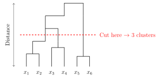
Advantages of Hierarchical Clustering:

• No need to specify \(K\) in advance

• Dendrogram provides full hierarchy

• Deterministic (no random initialization)

• Can handle any distance metric

• Intuitive visualization

Limitations:

• Computational cost: \(O(n^3)\) time, \(O(n^2)\) space

• Cannot scale to large datasets (millions of points)

• Greedy: Cannot undo merges

• Sensitive to noise and outliers

When to use:

• Small to medium datasets (\(n < 10,000\))

• When you want to explore different numbers of clusters

• When hierarchy itself is meaningful (taxonomy, phylogenetic trees)

19.3 DBSCAN (Density-Based Clustering)

Definition 19.8 (DBSCAN). DBSCAN (Density-Based Spatial Clustering of Applications with Noise) clusters based on density. Two parameters:

• \(\epsilon\): Neighborhood radius

• \(\text{minPts}\): Minimum points to form a dense region

Point types:

• Core point: Has \(\geq \text{minPts}\) points within distance \(\epsilon\)

• Border point: Within \(\epsilon\) of a core point, but not core itself

• Noise point: Neither core nor border

Algorithm Summary

DBSCAN Algorithm

Input: Data \(\{\boldsymbol{x}_i\}\), \(\epsilon\), \(\text{minPts}\)

Initialize: All points unmarked, cluster counter \(C = 0\)

For each unmarked point \(\boldsymbol{x}_i\):

1. Find \(N_\epsilon(\boldsymbol{x}_i) = \{\boldsymbol{x}_j : \left\lVert\boldsymbol{x}_i - \boldsymbol{x}_j\right\rVert \leq \epsilon\}\) (neighbors)

2. If \(|N_\epsilon(\boldsymbol{x}_i)| < \text{minPts}\):

   • Mark \(\boldsymbol{x}_i\) as noise (for now)

3. Else (\(\boldsymbol{x}_i\) is core point):

   • \(C = C + 1\) (new cluster)

   • Mark \(\boldsymbol{x}_i\) with cluster \(C\)

   • Initialize queue \(Q = N_\epsilon(\boldsymbol{x}_i)\)

   • While \(Q\) not empty:

     • Pop \(\boldsymbol{x}_j\) from \(Q\)

     • If \(\boldsymbol{x}_j\) was noise: mark with cluster \(C\) (border point)

     • If \(\boldsymbol{x}_j\) unmarked: mark with cluster \(C\)

     • If \(\boldsymbol{x}_j\) is core point: add its neighbors to \(Q\)

Output: Cluster assignments (or noise label)

DBSCAN finds arbitrarily-shaped clusters and identifies outliers as noise

Key Idea

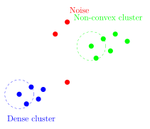
Advantages of DBSCAN:

• Discovers arbitrary shapes: Not limited to spherical clusters

• Handles noise: Explicitly identifies outliers

• No need to specify \(K\): Number of clusters determined automatically

• Only two parameters: \(\epsilon\) and minPts

Limitations:

• Sensitive to \(\epsilon\) and minPts (hard to tune)

• Struggles with varying densities

• \(O(n^2)\) complexity (can use KD-trees to reduce to \(O(n\log n)\))

• Border points can be assigned arbitrarily if equidistant to multiple clusters

Parameter selection:

• minPts: Often set to \(2d\) where \(d\) is dimensionality, or 4-5 for 2D data

• \(\epsilon\): Plot k-distance graph (distance to \(k\)-th nearest neighbor), look for “knee”

19.4 Cluster Evaluation Metrics

When ground truth labels are unavailable:

Definition 19.9 (Davies-Bouldin Index). \[\text{DB} = \frac{1}{K}\sum_{i=1}^K \max_{j \neq i} \left(\frac{s_i + s_j}{d_{ij}}\right)\] where \(s_i\) is average distance within cluster \(i\), and \(d_{ij}\) is distance between cluster centers.

Lower is better (smaller within-cluster spread, larger between-cluster separation).

Definition 19.10 (Calinski-Harabasz Index (Variance Ratio)). \[\text{CH} = \frac{\text{Between-cluster variance}}{\text{Within-cluster variance}} \cdot \frac{n - K}{K - 1}\] Higher is better (better separation).

When ground truth labels are available:

Definition 19.11 (Adjusted Rand Index (ARI)). Measures agreement between predicted clusters and true labels, adjusted for chance. \[\text{ARI} \in [-1, 1]\]

• ARI = 1: Perfect agreement

• ARI = 0: Random assignment

• ARI < 0: Worse than random

20 Dimensionality Reduction

20.1 Motivation

Key Idea

The Curse of Dimensionality:

• Data in high dimensions is sparse (most volume in corners of hypercube)

• Distance metrics become less meaningful

• Overfitting becomes severe

• Computational cost grows exponentially

Benefits of Dimensionality Reduction:

• Visualization (reduce to 2D or 3D)

• Noise reduction (eliminate irrelevant features)

• Faster training (fewer features)

• Storage efficiency

• Avoid overfitting

Two approaches:

• Feature Selection: Select subset of original features

• Feature Extraction: Create new features as combinations of originals

20.2 Principal Component Analysis (PCA)

20.2.1 Intuition and Formulation

Definition 20.1 (PCA Goal). Find a low-dimensional linear subspace that captures maximum variance in the data.

Formally, find \(k\) orthogonal directions \(\{\boldsymbol{u}_1, \ldots, \boldsymbol{u}_k\}\) that maximize: \[\max_{\boldsymbol{u}_1, \ldots, \boldsymbol{u}_k} \sum_{j=1}^k \mathrm{Var}(\boldsymbol{x}^\top \boldsymbol{u}_j)\] subject to \(\left\lVert\boldsymbol{u}_j\right\rVert = 1\) and \(\boldsymbol{u}_i \perp \boldsymbol{u}_j\) for \(i \neq j\).

Intuition 199. PCA finds new coordinate axes (principal components) along which data has maximum spread. The first component captures the most variance, the second captures the most remaining variance (orthogonal to the first), and so on.

Think of a 3D cloud of points shaped like a pancake. PCA finds the plane that best fits the pancake, and potentially a line within that plane.

Theorem 20.3 (PCA via Eigendecomposition). Given centered data (mean subtracted), the principal components are the eigenvectors of the covariance matrix \(\boldsymbol{\Sigma} = \frac{1}{n}\boldsymbol{X}^\top\boldsymbol{X}\).

Steps:

1. Center data: \(\tilde{\boldsymbol{x}}_i = \boldsymbol{x}_i - \bar{\boldsymbol{x}}\) where \(\bar{\boldsymbol{x}} = \frac{1}{n}\sum_i \boldsymbol{x}_i\)

2. Compute covariance: \(\boldsymbol{\Sigma} = \frac{1}{n}\sum_{i=1}^n \tilde{\boldsymbol{x}}_i\tilde{\boldsymbol{x}}_i^\top\)

3. Eigendecomposition: \(\boldsymbol{\Sigma} = \boldsymbol{U}\boldsymbol{\Lambda}\boldsymbol{U}^\top\)

4. Sort eigenvalues \(\lambda_1 \geq \lambda_2 \geq \cdots \geq \lambda_d\)

5. Top \(k\) eigenvectors \(\{\boldsymbol{u}_1, \ldots, \boldsymbol{u}_k\}\) are principal components

Projection: \(\boldsymbol{z}_i = \boldsymbol{U}_k^\top \tilde{\boldsymbol{x}}_i \in \mathbb{R}^k\) where \(\boldsymbol{U}_k = [\boldsymbol{u}_1, \ldots, \boldsymbol{u}_k]\).

Reconstruction: \(\hat{\boldsymbol{x}}_i = \boldsymbol{U}_k \boldsymbol{z}_i + \bar{\boldsymbol{x}}\).

Sketch. We want to maximize \(\sum_i (\boldsymbol{u}_1^\top \tilde{\boldsymbol{x}}_i)^2 = \boldsymbol{u}_1^\top \left(\sum_i \tilde{\boldsymbol{x}}_i\tilde{\boldsymbol{x}}_i^\top\right)\boldsymbol{u}_1 = \boldsymbol{u}_1^\top \boldsymbol{\Sigma} \boldsymbol{u}_1\).

Using Lagrange multipliers for constraint \(\left\lVert\boldsymbol{u}_1\right\rVert = 1\): \[\mathcal{L} = \boldsymbol{u}_1^\top \boldsymbol{\Sigma} \boldsymbol{u}_1 - \lambda(\boldsymbol{u}_1^\top\boldsymbol{u}_1 - 1)\] Taking derivative and setting to zero: \[\boldsymbol{\Sigma}\boldsymbol{u}_1 = \lambda\boldsymbol{u}_1\] So \(\boldsymbol{u}_1\) is an eigenvector of \(\boldsymbol{\Sigma}\). To maximize variance, choose eigenvector with largest eigenvalue \(\lambda_1\). The variance captured is \(\lambda_1\). Repeat for subsequent components (orthogonal eigenvectors). ◻

Algorithm Summary

PCA Algorithm

Input: Data \(\boldsymbol{X} \in \mathbb{R}^{n \times d}\), target dimension \(k\)

1. Center data: \(\tilde{\boldsymbol{X}} = \boldsymbol{X} - \bar{\boldsymbol{x}}\mathbf{1}^\top\) where \(\bar{\boldsymbol{x}} = \frac{1}{n}\sum_i \boldsymbol{x}_i\)

2. Compute covariance: \(\boldsymbol{\Sigma} = \frac{1}{n}\tilde{\boldsymbol{X}}^\top\tilde{\boldsymbol{X}}\)

3. Compute eigenvectors/eigenvalues: \(\boldsymbol{\Sigma} = \boldsymbol{U}\boldsymbol{\Lambda}\boldsymbol{U}^\top\)

4. Sort eigenvalues in descending order

5. Select top \(k\) eigenvectors: \(\boldsymbol{U}_k = [\boldsymbol{u}_1, \ldots, \boldsymbol{u}_k]\)

6. Project data: \(\boldsymbol{Z} = \tilde{\boldsymbol{X}}\boldsymbol{U}_k\)

Output: Reduced data \(\boldsymbol{Z} \in \mathbb{R}^{n \times k}\), transformation \(\boldsymbol{U}_k\)

20.2.2 Choosing Number of Components

Definition 20.4 (Explained Variance Ratio). Proportion of total variance captured by first \(k\) components: \[\text{EVR}_k = \frac{\sum_{j=1}^k \lambda_j}{\sum_{j=1}^d \lambda_j}\] Common threshold: Keep enough components to explain 90-95% of variance.

Scree plot: Cumulative explained variance vs number of components

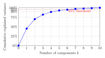
20.2.3 PCA Properties and Limitations

Key Idea

Key Properties of PCA:

• Linear transformation: \(\boldsymbol{z} = \boldsymbol{U}_k^\top(\boldsymbol{x} - \bar{\boldsymbol{x}})\)

• Optimal reconstruction: Minimizes reconstruction error \(\sum_i \left\lVert\boldsymbol{x}_i - \hat{\boldsymbol{x}}_i\right\rVert^2\)

• Uncorrelated components: \(\mathrm{Cov}(\boldsymbol{z}_i, \boldsymbol{z}_j) = 0\) for \(i \neq j\)

• Ordered by importance: First component captures most variance

Advantages:

• Fast, closed-form solution (eigendecomposition)

• Interpretable (variance explained)

• No hyperparameters (except \(k\))

• Reversible (can reconstruct)

Limitations:

• Linear only: Cannot capture non-linear structure

• Assumes variance = importance: High variance might be noise

• Sensitive to scaling: Must standardize features first

• Assumes Gaussian distribution: Works best for normally distributed data

• Interpretability: Components are linear combinations, hard to interpret

When to use PCA:

• Preprocessing for supervised learning

• Visualization (project to 2D/3D)

• Noise reduction

• When features are correlated

20.3 Linear Discriminant Analysis (LDA)

Definition 20.5 (LDA). Unlike PCA (unsupervised), LDA is supervised dimensionality reduction. It finds directions that maximize separation between classes.

Goal: Find projection \(\boldsymbol{w}\) that maximizes: \[J(\boldsymbol{w}) = \frac{\text{Between-class variance}}{\text{Within-class variance}} = \frac{\boldsymbol{w}^\top \boldsymbol{S}_B \boldsymbol{w}}{\boldsymbol{w}^\top \boldsymbol{S}_W \boldsymbol{w}}\] where:

• \(\boldsymbol{S}_W = \sum_{c=1}^K \sum_{i \in C_c} (\boldsymbol{x}_i - \boldsymbol{\mu}_c)(\boldsymbol{x}_i - \boldsymbol{\mu}_c)^\top\) (within-class scatter)

• \(\boldsymbol{S}_B = \sum_{c=1}^K n_c (\boldsymbol{\mu}_c - \boldsymbol{\mu})(\boldsymbol{\mu}_c - \boldsymbol{\mu})^\top\) (between-class scatter)

Theorem 20.6 (LDA Solution). Optimal projection directions are eigenvectors of \(\boldsymbol{S}_W^{-1}\boldsymbol{S}_B\) corresponding to largest eigenvalues.

Maximum number of components: \(\min(d, K-1)\) where \(K\) is number of classes.

Key Idea

PCA vs LDA:

• PCA: Unsupervised, maximizes variance, uses all data

• LDA: Supervised, maximizes class separation, uses labels

When to use LDA:

• Dimensionality reduction before classification

• When classes are well-separated

• When you have class labels

LDA often gives better results for classification tasks because it uses label information.

20.4 Non-Linear Methods

20.4.1 t-SNE (t-Distributed Stochastic Neighbor Embedding)

Definition 20.7 (t-SNE). Non-linear method that preserves local structure. Particularly good for visualization.

Idea:

1. In high-dimensional space, compute pairwise similarities: \[p_{ij} = \frac{\exp(-\left\lVert\boldsymbol{x}_i - \boldsymbol{x}_j\right\rVert^2 / 2\sigma^2)}{\sum_{k \neq l} \exp(-\left\lVert\boldsymbol{x}_k - \boldsymbol{x}_l\right\rVert^2 / 2\sigma^2)}\]

2. In low-dimensional space, use t-distribution: \[q_{ij} = \frac{(1 + \left\lVert\boldsymbol{z}_i - \boldsymbol{z}_j\right\rVert^2)^{-1}}{\sum_{k \neq l} (1 + \left\lVert\boldsymbol{z}_k - \boldsymbol{z}_l\right\rVert^2)^{-1}}\]

3. Minimize KL divergence: \(\text{KL}(P||Q) = \sum_{i,j} p_{ij}\log\frac{p_{ij}}{q_{ij}}\)

Optimized via gradient descent.

Key Idea

t-SNE Properties:

• Excellent for visualization (clusters become very clear)

• Preserves local structure (nearby points stay nearby)

• Non-linear (can capture complex manifolds)

• Stochastic (different runs give different results)

• Cannot be applied to new data (no explicit mapping, must rerun)

• Computationally expensive: \(O(n^2)\)

• Hyperparameter sensitive (perplexity, learning rate)

When to use:

• Visualization of high-dimensional data

• Exploratory analysis

• Not for preprocessing (use PCA for that)

Interpretation caution:

• Cluster sizes don’t mean anything

• Distances between clusters don’t mean anything

• Only local structure (within clusters) is meaningful

20.4.2 UMAP (Uniform Manifold Approximation and Projection)

Definition 20.8 (UMAP). Similar goal to t-SNE but with better theoretical foundation (Riemannian geometry and algebraic topology).

Advantages over t-SNE:

• Faster (\(O(n)\) vs \(O(n^2)\))

• Better preserves global structure

• Can be applied to new data (unlike t-SNE)

• Scales to larger datasets

• Often better separation of clusters

Popular for single-cell RNA-seq visualization and other large-scale applications.

20.4.3 Autoencoders

Definition 20.9 (Autoencoder). Neural network that learns to compress and reconstruct data.

Architecture:

• Encoder: \(\boldsymbol{z} = f_{\text{enc}}(\boldsymbol{x}; \boldsymbol{\theta}_{\text{enc}})\) maps \(\boldsymbol{x} \in \mathbb{R}^d\) to \(\boldsymbol{z} \in \mathbb{R}^k\) (bottleneck)

• Decoder: \(\hat{\boldsymbol{x}} = f_{\text{dec}}(\boldsymbol{z}; \boldsymbol{\theta}_{\text{dec}})\) reconstructs from \(\boldsymbol{z}\)

Training: Minimize reconstruction error: \[\mathcal{L}= \sum_{i=1}^n \left\lVert\boldsymbol{x}_i - \hat{\boldsymbol{x}}_i\right\rVert^2\]

Key Idea

Types of Autoencoders:

• Undercomplete: Bottleneck \(k < d\) (forced to compress)

• Sparse: Regularize activations in bottleneck

• Denoising: Train to reconstruct from corrupted input

• Variational (VAE): Learn probability distribution in latent space (generative model)

Advantages:

• Non-linear (can capture complex structure)

• Flexible architecture

• Can handle any data type (images, text, etc.)

• Can be applied to new data (just run encoder)

Limitations:

• Requires training (no closed form)

• Many hyperparameters

• Can be slow to train

• May overfit with limited data

21 Association Rule Learning

21.1 Market Basket Analysis

Definition 21.1 (Association Rules). Given transactions (sets of items), find rules of the form: \[X \Rightarrow Y\] meaning “if \(X\) is purchased, then \(Y\) is likely to be purchased.”

Example: \(\{\text{bread, butter}\} \Rightarrow \{\text{milk}\}\)

Definition 21.2 (Key Metrics). For rule \(X \Rightarrow Y\):

1. Support: \[\text{support}(X \Rightarrow Y) = P(X \cup Y) = \frac{\text{transactions containing } X \text{ and } Y}{\text{total transactions}}\] Measures how frequently the rule occurs.

2. Confidence: \[\text{confidence}(X \Rightarrow Y) = P(Y | X) = \frac{\text{support}(X \cup Y)}{\text{support}(X)}\] Measures reliability: if \(X\) is purchased, how often is \(Y\) also purchased?

3. Lift: \[\text{lift}(X \Rightarrow Y) = \frac{P(X \cup Y)}{P(X)P(Y)} = \frac{\text{confidence}(X \Rightarrow Y)}{\text{support}(Y)}\] Measures how much more likely \(Y\) is given \(X\) compared to \(Y\) alone.

• Lift > 1: \(X\) and \(Y\) are positively correlated

• Lift = 1: Independent

• Lift < 1: Negatively correlated

Example 21.3 (Market Basket). Store with 1000 transactions:

• Bread purchased: 600 times

• Milk purchased: 500 times

• Bread AND Milk: 400 times

For rule \(\{\text{bread}\} \Rightarrow \{\text{milk}\}\): \[\begin{align} \text{support} &= \frac{400}{1000} = 0.4 \\ \text{confidence} &= \frac{400}{600} = 0.67 \\ \text{lift} &= \frac{0.4}{0.6 \times 0.5} = 1.33 \end{align}\] People who buy bread are 33% more likely to buy milk than average.

21.2 Apriori Algorithm

Theorem 21.4 (Apriori Principle). If an itemset is frequent, then all of its subsets must also be frequent. Equivalently: \[\text{If } X \subseteq Y \text{ and } Y \text{ is infrequent, then } X \text{ is infrequent}\] This allows pruning the search space.

Algorithm Summary

Apriori Algorithm

Input: Transactions \(\mathcal{T}\), minimum support threshold \(\text{minsup}\)

Initialize: \(L_1 = \{\text{frequent 1-itemsets}\}\) (items with support \(\geq\) minsup)

For \(k = 2, 3, \ldots\) until \(L_k = \emptyset\):

1. Generate candidates: \(C_k = \text{generate}(L_{k-1})\)

   • Join pairs in \(L_{k-1}\) that share \(k-2\) items

   • Prune candidates whose \((k-1)\)-subsets are not in \(L_{k-1}\)

2. Count support: Scan database to count support of each candidate in \(C_k\)

3. Filter: \(L_k = \{c \in C_k : \text{support}(c) \geq \text{minsup}\}\)

Output: All frequent itemsets \(L = \bigcup_k L_k\)

Generate rules: For each frequent itemset \(X\), generate rules \(X \setminus Y \Rightarrow Y\) for all \(Y \subset X\) with sufficient confidence.

Key Idea

Apriori Advantages:

• Uses smart pruning to avoid checking all \(2^n\) itemsets

• Guarantees finding all rules above thresholds

• Simple and interpretable

Limitations:

• Multiple database scans (one per level)

• Generates many candidates

• Not efficient for very large databases or low support thresholds

FP-Growth: More efficient alternative

• Builds compressed data structure (FP-tree)

• Only 2 database scans

• No candidate generation

• Faster than Apriori, especially for large dense datasets

21.3 Applications

• Retail: Product placement, cross-selling, promotions

• Web usage mining: Page navigation patterns

• Bioinformatics: Gene co-occurrence, protein interactions

• Healthcare: Symptom associations, drug interactions

21.4 Summary of Part 5

1. Clustering: Group similar points. K-means for spherical clusters (fast but needs \(K\)). Hierarchical for dendrograms (intuitive but slow). DBSCAN for arbitrary shapes and noise handling.

2. Cluster Evaluation: Silhouette score, Davies-Bouldin index (intrinsic). ARI when ground truth available.

3. PCA: Linear dimensionality reduction via eigendecomposition. Maximizes variance, fast, but linear only. Use for preprocessing and visualization.

4. LDA: Supervised dimensionality reduction. Maximizes class separation. Better than PCA for classification tasks.

5. t-SNE: Non-linear visualization. Excellent for exploratory analysis but cannot be applied to new data. Preserves local structure only.

6. UMAP: Similar to t-SNE but faster, better global structure preservation, and can transform new data.

7. Autoencoders: Neural network-based non-linear reduction. Flexible but requires training.

8. Association Rules: Find patterns in transaction data. Apriori algorithm with support/confidence/lift metrics. Applications in retail and beyond.

Next Steps: Part 6 covers model evaluation, selection, hyperparameter tuning, and practical aspects of deploying ML systems.

Exercise 21.5.

1. For K-means with data \(\{(1,1), (1,2), (5,5), (5,6)\}\) and \(K=2\), starting with centroids at \((1,1)\) and \((5,5)\), perform one complete iteration (assignment + update). What are the new centroids?

2. Show that the K-means objective \(J\) decreases (or stays the same) in both the assignment step and the update step.

3. For hierarchical clustering with complete linkage, compute the dendrogram for points \(\{(0,0), (1,0), (0,1), (5,5)\}\) using Euclidean distance.

4. Given covariance matrix \(\boldsymbol{\Sigma} = \begin{bmatrix} 4 & 2 \\ 2 & 2 \end{bmatrix}\), find the principal components (eigenvectors) and explained variance (eigenvalues).

5. Explain why PCA requires centering the data (subtracting the mean). What happens if you don’t center?

6. For transactions: \(\{A,B,C\}, \{A,B\}, \{A,C\}, \{B,C\}, \{B\}\), find all rules with minimum support 0.4 and minimum confidence 0.6.

7. Compare computational complexity: K-means, hierarchical clustering (complete linkage), and DBSCAN. Which is fastest for \(n=100,000\) points?

8. When would you use t-SNE vs PCA vs UMAP? Give specific scenarios for each.

Part 6: Model Evaluation & Practical Aspects

22 Model Evaluation Metrics

22.1 Classification Metrics

22.1.1 Confusion Matrix

Definition 22.1 (Confusion Matrix). For binary classification with classes {Positive, Negative}:

		Predicted
3-4	Positive	Negative
2-4	Positive	TP	FN
2-4	Negative	FP	TN
2-4

where:

• TP (True Positive): Correctly predicted positive

• TN (True Negative): Correctly predicted negative

• FP (False Positive): Incorrectly predicted positive (Type I error)

• FN (False Negative): Incorrectly predicted negative (Type II error)

Example 22.2 (Medical Diagnosis). Disease detection model tested on 100 patients:

3-4	Predicted
3-4	Disease	Healthy
2-4	Disease	40	10
2-4	Healthy	5	45
2-4

TP=40 (correct disease detection), TN=45 (correct healthy), FP=5 (false alarm), FN=10 (missed disease).

22.1.2 Basic Metrics

Definition 22.3 (Classification Metrics). 1. Accuracy: \[\text{Accuracy} = \frac{TP + TN}{TP + TN + FP + FN}\] Proportion of correct predictions overall.

Limitation: Misleading for imbalanced datasets (e.g., 95% negative class \(\to\) predicting all negative gives 95% accuracy).

2. Precision (Positive Predictive Value): \[\text{Precision} = \frac{TP}{TP + FP}\] Of all predicted positives, what fraction are actually positive? “How precise are positive predictions?”

3. Recall (Sensitivity, True Positive Rate): \[\text{Recall} = \frac{TP}{TP + FN}\] Of all actual positives, what fraction did we detect? “How many positives did we recall?”

4. Specificity (True Negative Rate): \[\text{Specificity} = \frac{TN}{TN + FP}\] Of all actual negatives, what fraction did we correctly identify?

5. F1-Score (Harmonic Mean of Precision and Recall): \[F_1 = 2 \cdot \frac{\text{Precision} \cdot \text{Recall}}{\text{Precision} + \text{Recall}} = \frac{2TP}{2TP + FP + FN}\] Balances precision and recall. Useful when both are important.

6. F\(_\beta\)-Score (Generalized): \[F_\beta = (1 + \beta^2) \cdot \frac{\text{Precision} \cdot \text{Recall}}{\beta^2 \cdot \text{Precision} + \text{Recall}}\]

• \(\beta = 1\): Equal weight (F1)

• \(\beta > 1\): More weight on recall

• \(\beta < 1\): More weight on precision

Key Idea

Precision vs Recall Trade-off:

High Precision, Low Recall:

• Conservative predictions

• Few false alarms (FP), but miss many positives (FN)

• Example: Spam filter that rarely flags legitimate email as spam but misses some spam

High Recall, Low Precision:

• Aggressive predictions

• Catch most positives (low FN), but many false alarms (FP)

• Example: Cancer screening that detects most cases but has many false positives

When to prioritize:

• Precision: When false positives are costly (e.g., predicting customer will buy expensive item, spam detection)

• Recall: When false negatives are costly (e.g., disease detection, fraud detection)

• F1: When both matter equally

Example 22.4 (Computing Metrics). From medical diagnosis example (TP=40, TN=45, FP=5, FN=10): \[\begin{align} \text{Accuracy} &= \frac{40+45}{100} = 0.85 \\ \text{Precision} &= \frac{40}{40+5} = 0.889 \\ \text{Recall} &= \frac{40}{40+10} = 0.80 \\ \text{Specificity} &= \frac{45}{45+5} = 0.90 \\ F_1 &= 2 \cdot \frac{0.889 \cdot 0.80}{0.889 + 0.80} = 0.842 \end{align}\]

22.1.3 ROC Curve and AUC

Definition 22.5 (ROC Curve). The Receiver Operating Characteristic (ROC) curve plots:

• X-axis: False Positive Rate (FPR) = \(\frac{FP}{FP + TN} = 1 - \text{Specificity}\)

• Y-axis: True Positive Rate (TPR) = \(\frac{TP}{TP + FN} = \text{Recall}\)

at various classification thresholds.

For a classifier outputting probability \(p\), vary threshold \(t\): predict positive if \(p \geq t\).

ROC curves for different classifier qualities

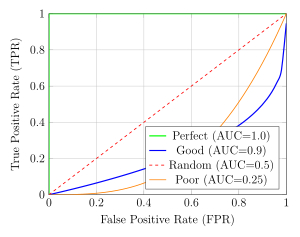
Definition 22.6 (AUC (Area Under the Curve)). AUC-ROC is the area under the ROC curve:

• AUC = 1.0: Perfect classifier (100% TPR, 0% FPR)

• AUC = 0.5: Random guessing (diagonal line)

• AUC < 0.5: Worse than random (invert predictions!)

Interpretation: Probability that the classifier ranks a random positive example higher than a random negative example.

Key Idea

Advantages of ROC-AUC:

• Threshold-independent: Evaluates all possible thresholds

• Robust to class imbalance: Unlike accuracy

• Single number summary: Easy to compare models

• Probabilistic interpretation: Ranking quality

When to use ROC vs PR:

• ROC: Balanced classes, care about both classes equally

• PR: Imbalanced classes, focus on positive class (more informative)

22.1.4 Precision-Recall Curve

Definition 22.7 (PR Curve). Plots Precision vs Recall at various thresholds.

Better for imbalanced datasets where positive class is rare.

PR curve: Better classifiers maintain high precision as recall increases

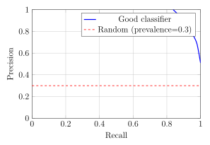
Definition 22.8 (AP and mAP). Average Precision (AP): Area under PR curve (approximation): \[AP = \sum_{k=1}^n (R_k - R_{k-1}) P_k\] where \(P_k\) and \(R_k\) are precision and recall at \(k\)-th threshold.

Mean Average Precision (mAP): Average AP across multiple classes (used in object detection).

22.1.5 Multi-Class Metrics

Definition 22.9 (Multi-Class Extension). For \(K\) classes, confusion matrix is \(K \times K\).

Macro-averaging: Compute metric for each class, then average (treats all classes equally). \[\text{Macro-F1} = \frac{1}{K}\sum_{k=1}^K F1_k\]

Micro-averaging: Pool all TP, FP, FN across classes, then compute metric (weights by class size). \[\text{Micro-Precision} = \frac{\sum_{k=1}^K TP_k}{\sum_{k=1}^K (TP_k + FP_k)}\]

Weighted-averaging: Weight each class metric by its support (number of true instances).

Key Idea

When to use:

• Macro: When all classes are equally important (regardless of size)

• Micro: When larger classes should dominate the metric

• Weighted: Balance between macro and micro, considering class sizes

For imbalanced datasets, macro-averaging can reveal poor performance on minority classes that micro-averaging might hide.

22.2 Regression Metrics

Definition 22.10 (Regression Metrics). For predictions \(\hat{y}_i\) and true values \(y_i\):

1. Mean Absolute Error (MAE): \[MAE = \frac{1}{n}\sum_{i=1}^n |y_i - \hat{y}_i|\] Average absolute difference. Robust to outliers, same units as \(y\).

2. Mean Squared Error (MSE): \[MSE = \frac{1}{n}\sum_{i=1}^n (y_i - \hat{y}_i)^2\] Penalizes large errors heavily. Not in original units.

3. Root Mean Squared Error (RMSE): \[RMSE = \sqrt{MSE} = \sqrt{\frac{1}{n}\sum_{i=1}^n (y_i - \hat{y}_i)^2}\] Same scale as \(y\). More interpretable than MSE.

4. Mean Absolute Percentage Error (MAPE): \[MAPE = \frac{100\%}{n}\sum_{i=1}^n \left|\frac{y_i - \hat{y}_i}{y_i}\right|\] Scale-independent. Undefined when \(y_i = 0\).

5. R² (Coefficient of Determination): \[R^2 = 1 - \frac{SS_{\text{res}}}{SS_{\text{tot}}} = 1 - \frac{\sum_i(y_i - \hat{y}_i)^2}{\sum_i(y_i - \bar{y})^2}\] where \(\bar{y} = \frac{1}{n}\sum_i y_i\).

• \(R^2 = 1\): Perfect predictions

• \(R^2 = 0\): Model no better than predicting mean

• \(R^2 < 0\): Model worse than mean (possible with non-linear models)

Measures proportion of variance explained by the model.

Key Idea

MAE vs MSE/RMSE:

• MAE:

  • Robust to outliers

  • All errors weighted equally

  • Easier to interpret

• MSE/RMSE:

  • Sensitive to outliers (large errors penalized heavily)

  • Differentiable everywhere (better for optimization)

  • Common in statistical theory

When outliers matter: Use MAE

When large errors are particularly bad: Use MSE/RMSE

R² advantages:

• Scale-independent (compare across different problems)

• Intuitive (percentage of variance explained)

R² limitations:

• Always increases with more features (use adjusted R²)

• Can be negative for non-linear models

• Doesn’t indicate if model is appropriate

23 Model Selection and Hyperparameter Tuning

23.1 Cross-Validation

23.1.1 K-Fold Cross-Validation

Definition 23.1 (K-Fold Cross-Validation). Split data into \(K\) equal-sized folds. For each fold \(k\):

1. Train on folds \(\{1, \ldots, K\} \setminus \{k\}\)

2. Validate on fold \(k\)

3. Record validation metric \(M_k\)

Report average: \(\text{CV Score} = \frac{1}{K}\sum_{k=1}^K M_k\)

Common: \(K = 5\) or \(K = 10\).

5-fold cross-validation: Each fold serves as validation set once

Algorithm Summary

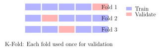
K-Fold Cross-Validation

Input: Data \(\mathcal{D}\), model/hyperparameters, \(K\)

1. Split \(\mathcal{D}\) into \(K\) equal-sized folds: \(\{\mathcal{D}_1, \ldots, \mathcal{D}_K\}\)

2. For \(k = 1\) to \(K\):

   • \(\mathcal{D}_{\text{train}} = \mathcal{D} \setminus \mathcal{D}_k\)

   • \(\mathcal{D}_{\text{val}} = \mathcal{D}_k\)

   • Train model on \(\mathcal{D}_{\text{train}}\)

   • Evaluate on \(\mathcal{D}_{\text{val}}\), record score \(M_k\)

3. Compute average score: \(\bar{M} = \frac{1}{K}\sum_{k=1}^K M_k\)

4. (Optional) Compute standard deviation: \(\sigma_M = \sqrt{\frac{1}{K}\sum_{k=1}^K (M_k - \bar{M})^2}\)

Output: Mean score \(\bar{M}\) and std \(\sigma_M\)

Key Idea

Why Cross-Validation?

Problem with single train/val split:

• High variance (depends on random split)

• Wastes data (validation set not used for training)

• May not be representative

CV advantages:

• Lower variance estimate

• Uses all data for both training and validation

• Provides confidence interval (via standard deviation)

• More reliable for model selection

Choosing \(K\):

• Small \(K\) (e.g., 3): Faster, higher bias, higher variance

• Large \(K\) (e.g., 10): Slower, lower bias, can have higher variance

• \(K = n\) (LOOCV): Maximum data per fold, very slow, high variance

• Common choice: \(K = 5\) or \(10\) (good trade-off)

23.1.2 Stratified K-Fold

Definition 23.2 (Stratified K-Fold). For classification, ensure each fold has approximately the same class distribution as the full dataset.

Particularly important for:

• Imbalanced datasets

• Small datasets

• Multi-class problems

Example 23.3 (Stratified Split). Dataset: 100 examples, 80 class A, 20 class B (80/20 split).

Regular 5-fold: Some folds might have 70/30 or 90/10 (random variation).

Stratified 5-fold: Each fold has exactly 16 class A, 4 class B (80/20 maintained).

23.1.3 Time Series Cross-Validation

Definition 23.4 (Time Series Split). For temporal data, cannot randomly shuffle (violates temporal order).

Forward chaining:

• Fold 1: Train on \([1:n_1]\), validate on \([n_1+1:n_2]\)

• Fold 2: Train on \([1:n_2]\), validate on \([n_2+1:n_3]\)

• Fold 3: Train on \([1:n_3]\), validate on \([n_3+1:n_4]\)

• ...

Always train on past, predict future (no data leakage).

23.2 Hyperparameter Tuning

23.2.1 Grid Search

Definition 23.5 (Grid Search). Exhaustively search over a specified hyperparameter grid.

Example: For SVM with RBF kernel:

• \(C \in \{0.1, 1, 10, 100\}\)

• \(\gamma \in \{0.001, 0.01, 0.1, 1\}\)

Test all \(4 \times 4 = 16\) combinations.

Algorithm Summary

Grid Search with Cross-Validation

Input: Training data \(\mathcal{D}\), model, hyperparameter grid, \(K\) for CV

1. Generate all combinations of hyperparameters from grid

2. For each combination \(\theta\):

   • Run \(K\)-fold CV with hyperparameters \(\theta\)

   • Record mean CV score \(\bar{M}(\theta)\)

3. Select best: \(\theta^* = \mathop{\mathrm{arg\,max}}_\theta \bar{M}(\theta)\)

4. Retrain final model on all data with \(\theta^*\)

Output: Best hyperparameters \(\theta^*\), trained model

Key Idea

Grid Search Advantages:

• Simple, easy to implement

• Guaranteed to find best combination in grid

• Parallelizable (each combination independent)

• Reproducible

Limitations:

• Curse of dimensionality: \(n\) parameters with \(k\) values each \(\to\) \(k^n\) combinations

• Wastes computation on unpromising regions

• Grid may miss optimal values between grid points

• Expensive for large grids or slow models

Best practices:

• Start with coarse grid, then refine around best values

• Use logarithmic spacing for parameters spanning orders of magnitude

• Limit grid size (test 3-5 values per parameter max)

23.2.2 Random Search

Definition 23.6 (Random Search). Sample hyperparameter combinations randomly from specified distributions.

Instead of grid, define distributions:

• \(C \sim \text{LogUniform}(10^{-3}, 10^3)\)

• \(\gamma \sim \text{LogUniform}(10^{-4}, 10^1)\)

Sample \(n\) random combinations, evaluate each.

Theorem 23.7 (Random Search Efficiency). Random search is often more efficient than grid search because:

• Some hyperparameters matter more than others

• Random search explores more unique values for important parameters

• With same budget, covers search space better

For \(n\) trials:

• Grid search with 2 parameters: \(\sqrt{n} \times \sqrt{n}\) grid

• Random search: \(n\) unique values per parameter

Grid vs Random search: Random explores more values for important parameter

Implementation Notes

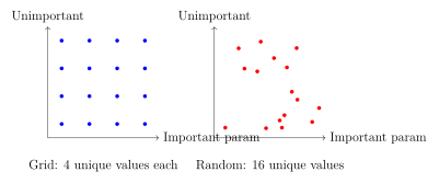
Random Search in Practice:

from sklearn.model_selection import RandomizedSearchCV
from scipy.stats import loguniform, randint

# Define distributions
param_distributions = {
    'C': loguniform(1e-3, 1e3),
    'gamma': loguniform(1e-4, 1e1),
    'kernel': ['rbf', 'poly']
}

# Random search with 100 iterations
random_search = RandomizedSearchCV(
    estimator=SVC(),
    param_distributions=param_distributions,
    n_iter=100,  # number of random samples
    cv=5,
    random_state=42,
    n_jobs=-1  # parallel
)

random_search.fit(X_train, y_train)
best_params = random_search.best_params_

23.2.3 Bayesian Optimization

Definition 23.8 (Bayesian Optimization). Intelligent search that uses past evaluations to guide future trials.

Key idea:

1. Build probabilistic model (surrogate) of \(f(\theta)\) where \(\theta\) are hyperparameters

2. Use model to select promising \(\theta\) (acquisition function)

3. Evaluate \(f(\theta)\), update model

4. Repeat

Common surrogate: Gaussian Process (GP)

Common acquisition functions:

• Expected Improvement (EI): Balance exploration/exploitation

• Upper Confidence Bound (UCB): \(\mu(\theta) + \kappa\sigma(\theta)\)

Key Idea

Bayesian Optimization vs Random/Grid:

Advantages:

• Much more sample-efficient (fewer evaluations needed)

• Learns from past trials

• Handles expensive black-box functions well

• Can incorporate prior knowledge

Disadvantages:

• More complex to implement

• Overhead in building surrogate model

• Less parallelizable

• Can get stuck in local optima

When to use:

• Expensive evaluations (training takes hours)

• Limited budget (can only try 10-50 configurations)

• Continuous hyperparameters

• Black-box optimization

Popular libraries: Optuna, Hyperopt, Scikit-Optimize, Ray Tune

23.3 Nested Cross-Validation

Definition 23.9 (Nested CV). For unbiased performance estimation with hyperparameter tuning:

Outer loop (performance estimation):

• \(K_{\text{outer}}\)-fold CV

Inner loop (hyperparameter selection):

• For each outer fold, run \(K_{\text{inner}}\)-fold CV on training portion

• Select best hyperparameters

• Evaluate on outer fold’s validation set

This prevents optimistic bias from tuning on the same data used for evaluation.

Nested CV: Inner loop tunes hyperparameters, outer loop evaluates performance

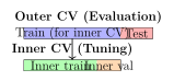
24 Data Preprocessing

24.1 Feature Scaling

24.1.1 Standardization (Z-score Normalization)

Definition 24.1 (Standardization). Transform features to have mean 0 and standard deviation 1: \[x_{\text{scaled}} = \frac{x - \mu}{\sigma}\] where \(\mu = \frac{1}{n}\sum_i x_i\) and \(\sigma = \sqrt{\frac{1}{n}\sum_i (x_i - \mu)^2}\).

Result: \(x_{\text{scaled}} \sim \mathcal{N}(0, 1)\) if original data is Gaussian.

Definition 24.2 (Min-Max Normalization). Scale features to a fixed range, typically \([0, 1]\): \[x_{\text{scaled}} = \frac{x - x_{\min}}{x_{\max} - x_{\min}}\]

For range \([a, b]\): \[x_{\text{scaled}} = a + (b - a) \cdot \frac{x - x_{\min}}{x_{\max} - x_{\min}}\]

Key Idea

When to use which:

Standardization:

• Features have different units/scales

• Many ML algorithms (SVM, logistic regression, neural networks)

• When outliers should not be emphasized

• Preserves outlier information (can go beyond \([0,1]\))

Min-Max:

• Need bounded range (e.g., \([0,1]\))

• Neural networks (especially with bounded activations like sigmoid)

• Image data (pixel values)

• When you want to preserve zero values

When NOT to scale:

• Tree-based models (decision trees, random forests, XGBoost)—invariant to monotonic transformations

• Features already on same scale

• Interpretability matters (keep original units)

Implementation Notes

Critical: Fit on Training, Transform on Test

from sklearn.preprocessing import StandardScaler

# Correct way
scaler = StandardScaler()
X_train_scaled = scaler.fit_transform(X_train)
X_test_scaled = scaler.transform(X_test)  # Use training statistics

# Wrong way (data leakage!)
# scaler.fit(X_test)  # Never fit on test data!

Why? Test data should be completely unseen. Using test statistics would leak information.

24.2 Encoding Categorical Variables

24.2.1 Label Encoding

Definition 24.3 (Label Encoding). Map categories to integers: \[\text{Red} \to 0, \quad \text{Green} \to 1, \quad \text{Blue} \to 2\]

Issue: Introduces artificial ordering (\(\text{Blue} > \text{Green} > \text{Red}\)).

When to use:

• Ordinal variables (Low \(<\) Medium \(<\) High)

• Tree-based models (can split on integers)

• Target variable in classification

24.2.2 One-Hot Encoding

Definition 24.4 (One-Hot Encoding). Create binary column for each category:

Original	Red	Green	Blue
Red	1	0	0
Green	0	1	0
Blue	0	0	1

For \(K\) categories, creates \(K\) binary features (or \(K-1\) to avoid multicollinearity).

Key Idea

One-Hot Advantages:

• No artificial ordering

• Works with linear models

• Standard approach for neural networks

Limitations:

• High cardinality: Many categories \(\to\) many features

• Sparse matrices: Most values are 0

• Curse of dimensionality: \(K\) categories = \(K\) new dimensions

Alternatives for high cardinality:

• Target encoding: Replace category with mean target value

• Frequency encoding: Replace with category frequency

• Embedding layers: Neural network learns dense representations (NLP, RecSys)

• Hashing trick: Hash categories to fixed number of buckets

24.3 Handling Missing Data

Definition 24.5 (Types of Missingness). 1. MCAR (Missing Completely At Random):

• Missingness independent of observed and unobserved data

• Example: Survey responses lost due to server crash

2. MAR (Missing At Random):

• Missingness depends on observed data, not unobserved

• Example: Older people less likely to report income (age is observed)

3. MNAR (Missing Not At Random):

• Missingness depends on unobserved data

• Example: High earners don’t report income (income itself causes missingness)

Definition 24.6 (Handling Strategies). 1. Deletion:

• Listwise: Remove entire row if any feature missing

• Pairwise: Use available data for each analysis

• When: MCAR, small amount of missing data (\(<\) 5%)

2. Imputation:

• Mean/Median/Mode: Simple, fast, but ignores relationships

• Forward/Backward fill: For time series

• KNN imputation: Use \(k\) nearest neighbors’ values

• Model-based: Regression, EM algorithm, MICE

• Indicator variable: Add binary flag for missingness (preserves information)

3. Model-Specific:

• Some algorithms handle missing values natively (XGBoost, LightGBM)

Implementation Notes

Imputation Best Practices:

from sklearn.impute import SimpleImputer, KNNImputer

# Simple imputation
imputer = SimpleImputer(strategy='mean')  # or 'median', 'most_frequent'
X_train_imputed = imputer.fit_transform(X_train)
X_test_imputed = imputer.transform(X_test)

# KNN imputation (more sophisticated)
knn_imputer = KNNImputer(n_neighbors=5)
X_train_imputed = knn_imputer.fit_transform(X_train)

Remember: Always fit imputer on training data only!

24.4 Outlier Detection and Treatment

Definition 24.7 (Outlier Detection Methods). 1. Statistical:

• Z-score: \(|z| > 3\) (assuming Gaussian)

• IQR method: Below \(Q_1 - 1.5 \cdot IQR\) or above \(Q_3 + 1.5 \cdot IQR\)

2. Distance-based:

• DBSCAN: Points marked as noise

• KNN: Points with large distance to \(k\)-th neighbor

3. Model-based:

• Isolation Forest: Isolates outliers in random trees

• One-Class SVM: Learns boundary around normal data

• Local Outlier Factor (LOF): Compares local density

Key Idea

Handling Outliers:

1. Investigate first:

• Data error (typo, measurement error)? → Correct or remove

• Valid extreme value? → Keep (important information)

2. Treatment options:

• Keep: If valid and informative

• Remove: If errors or not representative

• Cap/Winsorize: Replace with threshold (e.g., 95th percentile)

• Transform: Log, square root to reduce impact

• Separate model: Build model specifically for outliers

3. Model robustness:

• Robust models: Tree-based methods, robust regression (Huber loss)

• Sensitive models: Linear regression, KNN, SVM (need preprocessing)

25 Feature Engineering

25.1 Feature Extraction vs Selection

Definition 25.1 (Feature Engineering). Feature Extraction: Create new features from existing ones

• PCA: Linear combinations

• Polynomial features: \(x_1 \cdot x_2\), \(x_1^2\)

• Domain-specific transformations

Feature Selection: Choose subset of existing features

• Remove irrelevant or redundant features

• Improve model performance and interpretability

• Reduce overfitting and training time

25.2 Feature Selection Methods

25.2.1 Filter Methods

Definition 25.2 (Filter Methods). Select features based on statistical measures, independent of model.

1. Correlation: Remove features highly correlated with each other (redundant).

2. Mutual Information: \[MI(X, Y) = \sum_{x,y} P(x,y) \log\frac{P(x,y)}{P(x)P(y)}\] Measures dependence between feature and target (captures non-linear relationships).

3. Chi-Square Test: For categorical features and classification: \[\chi^2 = \sum_{i,j} \frac{(O_{ij} - E_{ij})^2}{E_{ij}}\] Tests independence between feature and target.

4. ANOVA F-test: For continuous features and categorical target. Tests if feature means differ across classes.

Key Idea

Filter Methods:

Advantages:

• Fast (no model training)

• Model-agnostic

• Good for preprocessing

Limitations:

• Ignores feature interactions

• Doesn’t consider model performance

• May select redundant features

25.2.2 Wrapper Methods

Definition 25.3 (Wrapper Methods). Use model performance to guide feature selection.

1. Forward Selection:

1. Start with no features

2. Add one feature at a time (choose best improvement)

3. Stop when no improvement

2. Backward Elimination:

1. Start with all features

2. Remove one feature at a time (remove worst)

3. Stop when removal hurts performance

3. Recursive Feature Elimination (RFE):

1. Train model on all features

2. Rank features by importance

3. Remove least important

4. Repeat until desired number of features

Algorithm Summary

Recursive Feature Elimination (RFE)

Input: Features \(\boldsymbol{X}\), target \(\boldsymbol{y}\), model, target feature count \(k\)

Initialize: Current feature set \(\mathcal{F} = \{\text{all features}\}\)

While \(|\mathcal{F}| > k\):

1. Train model on features in \(\mathcal{F}\)

2. Compute feature importances (e.g., coefficients, Gini importance)

3. Remove feature with lowest importance from \(\mathcal{F}\)

Output: Selected features \(\mathcal{F}\)

Key Idea

Wrapper Methods:

Advantages:

• Considers model performance directly

• Can capture feature interactions

• Optimizes for specific model

Limitations:

• Computationally expensive (many model trainings)

• Risk of overfitting (especially with small data)

• Model-specific (selected features may not work for other models)

25.2.3 Embedded Methods

Definition 25.4 (Embedded Methods). Feature selection built into model training.

1. L1 Regularization (Lasso): Penalty \(\lambda\sum_j |w_j|\) drives some weights to exactly zero.

2. Tree-based Feature Importance: Random Forest, XGBoost provide importance scores. Select top \(k\) features.

3. ElasticNet: Combines L1 (sparsity) and L2 (grouping) penalties.

Key Idea

Embedded Methods:

Advantages:

• Faster than wrapper methods

• Less overfitting risk

• Integrated with training

Best Practice:

1. Start with filter methods (fast preprocessing)

2. Use embedded methods if model supports (L1, tree importance)

3. Use wrapper methods for critical applications with budget

25.3 Domain-Specific Feature Engineering

Example 25.5 (Common Transformations). 1. Time Features (from datetime):

• Hour, day of week, month, year

• Is weekend? Is holiday?

• Time since event

• Cyclic encoding: \(\sin(2\pi \cdot \text{hour}/24)\), \(\cos(2\pi \cdot \text{hour}/24)\)

2. Text Features:

• Bag of words, TF-IDF

• N-grams

• Length, number of words, capitals

• Sentiment scores

• Word embeddings (Word2Vec, GloVe)

3. Geospatial:

• Distance to landmark

• Cluster of locations

• Urban vs rural classification

4. Interaction Features:

• Products: \(x_1 \cdot x_2\)

• Ratios: \(x_1 / x_2\)

• Differences: \(x_1 - x_2\)

5. Aggregations (for grouped data):

• Mean, median, std per group

• Count, min, max per group

• Time-based: rolling averages, lag features

25.4 Summary of Part 6

1. Classification Metrics: Confusion matrix, precision, recall, F1. ROC-AUC for balanced data, PR curve for imbalanced. Choose metric based on cost of errors.

2. Regression Metrics: MAE (robust to outliers), RMSE (penalizes large errors), R² (variance explained). Choose based on error characteristics.

3. Cross-Validation: K-fold for robust evaluation. Stratified for classification. Time series split for temporal data. Nested CV for hyperparameter tuning.

4. Hyperparameter Tuning: Grid search (exhaustive), random search (efficient), Bayesian optimization (sample-efficient for expensive evaluations).

5. Feature Scaling: Standardization (most ML algorithms), Min-Max (bounded activations). Always fit on training, transform on test.

6. Categorical Encoding: Label for ordinal, one-hot for nominal. Target encoding for high cardinality.

7. Missing Data: Understand missingness type (MCAR/MAR/MNAR). Imputation strategies from simple (mean) to complex (KNN, model-based).

8. Feature Selection: Filter (fast, model-agnostic), wrapper (model-specific, expensive), embedded (integrated). Use based on computational budget and goals.

Next Steps: Part 7 covers practical tools and deployment: WEKA, scikit-learn pipelines, and model serving strategies.

Exercise 25.6.

1. Given confusion matrix with TP=85, TN=40, FP=10, FN=15, compute accuracy, precision, recall, F1, and specificity.

2. Explain why accuracy is misleading for a dataset with 95% negative class, 5% positive class. What metrics would you use instead?

3. For a cancer detection model, would you prioritize precision or recall? Justify your answer and suggest an appropriate threshold strategy.

4. Implement 5-fold cross-validation by hand for a dataset with 100 examples. Show which examples go in which fold.

5. Why must we fit the scaler on training data only? What happens if we fit on all data (train + test)?

6. Design one-hot encoding for categorical variable {Red, Green, Blue, Red, Green}. How many columns? Should you use \(K\) or \(K-1\) columns?

7. Compare computational complexity: Grid search with 4 parameters (5 values each) vs random search with 100 iterations. Which tries more unique combinations for each parameter?

8. For time series data, why can’t we use regular k-fold cross-validation? Design a proper time series CV scheme for 120 monthly observations.

Part 7: Tools, Pipelines, and Deployment

26 WEKA: Practical Guide

26.1 Introduction to WEKA

Definition 26.1 (WEKA). WEKA (Waikato Environment for Knowledge Analysis) is a collection of machine learning algorithms for data mining tasks. Developed at University of Waikato, New Zealand.

Key Features:

• GUI-based interface (no coding required)

• Extensive algorithm library (classification, regression, clustering, etc.)

• Built-in visualization tools

• Java-based (cross-platform)

• Free and open-source

When to use WEKA:

• Quick prototyping and experimentation

• Teaching and learning ML concepts

• Comparing multiple algorithms easily

• Small to medium datasets

• When GUI is preferred over coding

26.2 WEKA Explorer Interface

Key Idea

WEKA Explorer has 6 main tabs:

1. Preprocess: Load data, view statistics, apply filters

• Import ARFF, CSV, JDBC databases

• View attribute statistics and distributions

• Apply filters (discretization, normalization, attribute selection)

2. Classify: Train classification/regression models

• Choose algorithm from tree structure

• Configure hyperparameters

• Select test options (cross-validation, percentage split, etc.)

• View results: accuracy, confusion matrix, ROC

3. Cluster: Perform clustering

• K-means, EM, DBSCAN, hierarchical

• Evaluate clusters

• Visualize assignments

4. Associate: Find association rules

• Apriori, FP-Growth

• Set minimum support and confidence

5. Select attributes: Feature selection

• Various search and evaluation methods

• Rank features by importance

6. Visualize: Data exploration

• Scatter plots, histograms

• Class distributions

• Interactive exploration

26.3 Data Format: ARFF

Definition 26.2 (ARFF Format). ARFF (Attribute-Relation File Format) is WEKA’s native format.

Structure:

@relation weather

@attribute outlook {sunny, overcast, rainy}
@attribute temperature numeric
@attribute humidity numeric
@attribute windy {TRUE, FALSE}
@attribute play {yes, no}

@data
sunny,85,85,FALSE,no
sunny,80,90,TRUE,no
overcast,83,86,FALSE,yes
rainy,70,96,FALSE,yes
...

Components:

• @relation: Dataset name

• @attribute: Feature name and type (numeric, nominal, string, date)

• @data: Actual data rows

26.4 Workflow Example: Classification

Algorithm Summary

WEKA Classification Workflow

Step 1: Load Data

• Open Explorer \(\to\) Preprocess tab

• Click “Open file...” \(\to\) Select ARFF or CSV

• Review attributes in the table

• Check class distribution (click on class attribute)

Step 2: Preprocess (Optional)

• Apply filters: Click “Choose” under Filter

• Example: unsupervised.attribute.Normalize for scaling

• Click “Apply” to execute filter

Step 3: Select Algorithm

• Click “Classify” tab

• Click “Choose” button

• Navigate tree: e.g., trees \(\to\) J48 (decision tree)

• Click on algorithm name to configure parameters

Step 4: Choose Test Method

• Cross-validation: Select folds (default 10)

• Percentage split: e.g., 66% train, 34% test

• Use training set: Evaluate on training (overfitting check)

• Supplied test set: Load separate test file

Step 5: Run and Evaluate

• Click “Start” button

• View results in output area:

  • Summary statistics

  • Confusion matrix

  • Detailed accuracy by class

• Right-click on result \(\to\) Visualize for plots

Step 6: Compare Models

• Run multiple algorithms (results stack in result list)

• Right-click result list \(\to\) Compare to compare

• Export results: Right-click \(\to\) Save result buffer

26.5 Common WEKA Algorithms

Common algorithms in WEKA by category

Category	Algorithms in WEKA
Trees	J48 (C4.5), RandomForest, REPTree
Rules	JRip, PART, DecisionTable
Functions	Logistic, MultilayerPerceptron, SMO (SVM)
Lazy	IBk (KNN), LWL
Bayes	NaiveBayes, BayesNet
Meta	AdaBoostM1, Bagging, Stacking, Vote
Clustering	SimpleKMeans, EM, DBSCAN, HierarchicalClusterer

26.6 Visualizing Results

Key Idea

WEKA Visualization Tools:

1. ROC Curve:

• After classification: Right-click result \(\to\) Visualize threshold curve

• Choose class and metric (TPR vs FPR for ROC)

• Compare multiple classifiers on same plot

2. Classification Errors:

• Right-click result \(\to\) Visualize classifier errors

• Shows 2D plot of predictions

• Misclassified instances highlighted

• Interactive: hover for details

3. Tree Visualization:

• After training tree (J48, RandomForest): Right-click \(\to\) Visualize tree

• Shows decision rules graphically

• Can save as PNG/PDF

4. Cost/Benefit Analysis:

• Define cost matrix for different types of errors

• WEKA computes expected cost

• Useful for imbalanced datasets

26.7 Advantages and Limitations

Key Idea

WEKA Advantages:

• Easy to use: GUI-based, no programming required

• Comprehensive: 100+ algorithms built-in

• Educational: Excellent for learning ML

• Visualization: Good built-in plots

• Reproducible: Can save configurations

WEKA Limitations:

• Not for production: GUI-based, not suitable for deployment

• Scalability: Limited to datasets that fit in memory

• Modern algorithms: Lacks latest methods (no XGBoost, deep learning)

• Automation: Difficult to automate workflows

• Customization: Limited compared to programming libraries

Best Use Cases:

• Academic research and teaching

• Quick baseline comparisons

• Data exploration

• Proof of concept

When to move beyond WEKA:

• Large-scale datasets (\(>\)1M rows)

• Production deployment

• Need for latest algorithms

• Complex preprocessing pipelines

• Integration with other systems

27 ML Pipelines in Python

27.1 Introduction to Scikit-learn

Definition 27.1 (Scikit-learn). Scikit-learn is Python’s premier machine learning library, offering:

• Consistent API across algorithms

• Comprehensive algorithm coverage

• Excellent documentation

• Integration with NumPy, Pandas, Matplotlib

• Production-ready code

Core API: All estimators follow the same pattern:

model = Estimator()          # Initialize
model.fit(X_train, y_train)  # Train
predictions = model.predict(X_test)  # Predict
score = model.score(X_test, y_test)  # Evaluate

27.2 The Pipeline Concept

Definition 27.2 (Pipeline). A Pipeline chains multiple processing steps into a single estimator: \[\text{Data} \xrightarrow{\text{Transform 1}} \xrightarrow{\text{Transform 2}} \xrightarrow{\cdots} \xrightarrow{\text{Model}}\]

Benefits:

• Convenience: Single fit()/predict() call

• Prevents leakage: Transformers fit only on training data

• Hyperparameter tuning: Tune entire pipeline with GridSearchCV

• Reproducibility: Easy to save and load entire workflow

• Code cleanliness: Organized preprocessing + modeling

Pipeline chains preprocessing and modeling steps

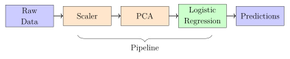
27.3 Building Pipelines

Implementation Notes

Basic Pipeline Example:

from sklearn.pipeline import Pipeline
from sklearn.preprocessing import StandardScaler
from sklearn.decomposition import PCA
from sklearn.linear_model import LogisticRegression

# Create pipeline
pipeline = Pipeline([
    ('scaler', StandardScaler()),      # Step 1: Scale
    ('pca', PCA(n_components=10)),     # Step 2: Reduce dim
    ('classifier', LogisticRegression()) # Step 3: Classify
])

# Use like any other estimator
pipeline.fit(X_train, y_train)
predictions = pipeline.predict(X_test)
accuracy = pipeline.score(X_test, y_test)

print(f"Accuracy: {accuracy:.3f}")

Key Points:

• Each step is a tuple: (’name’, transformer)

• All steps except last must have fit_transform()

• Last step must have fit() and predict()

• Access steps: pipeline.named_steps[’scaler’]

27.4 Column Transformer

Definition 27.3 (ColumnTransformer). Apply different transformations to different columns:

from sklearn.compose import ColumnTransformer
from sklearn.preprocessing import StandardScaler, OneHotEncoder

# Define transformations for different column types
preprocessor = ColumnTransformer([
    ('num', StandardScaler(), ['age', 'income']),
    ('cat', OneHotEncoder(), ['gender', 'city'])
])

# Use in pipeline
pipeline = Pipeline([
    ('preprocessor', preprocessor),
    ('classifier', RandomForestClassifier())
])

Benefits:

• Handle mixed data types (numerical + categorical)

• Apply appropriate transformation to each feature type

• Cleaner than manual column splitting

27.5 Pipeline with GridSearchCV

Implementation Notes

Hyperparameter Tuning with Pipeline:

from sklearn.model_selection import GridSearchCV

# Create pipeline
pipeline = Pipeline([
    ('scaler', StandardScaler()),
    ('classifier', SVC())
])

# Define parameter grid (use double underscore)
param_grid = {
    'classifier__C': [0.1, 1, 10],
    'classifier__gamma': [0.001, 0.01, 0.1],
    'classifier__kernel': ['rbf', 'linear']
}

# Grid search on entire pipeline
grid_search = GridSearchCV(
    pipeline, 
    param_grid, 
    cv=5, 
    scoring='accuracy',
    n_jobs=-1
)

grid_search.fit(X_train, y_train)

print(f"Best params: {grid_search.best_params_}")
print(f"Best CV score: {grid_search.best_score_:.3f}")

# Use best model
best_model = grid_search.best_estimator_
test_score = best_model.score(X_test, y_test)

Naming convention: Use step_name__parameter_name to reference pipeline parameters.

27.6 Custom Transformers

Definition 27.4 (Custom Transformer). Create your own transformer by inheriting from BaseEstimator and TransformerMixin:

from sklearn.base import BaseEstimator, TransformerMixin

class LogTransformer(BaseEstimator, TransformerMixin):
    def __init__(self, features):
        self.features = features
    
    def fit(self, X, y=None):
        return self  # Nothing to learn
    
    def transform(self, X):
        X_copy = X.copy()
        X_copy[self.features] = np.log1p(X_copy[self.features])
        return X_copy

# Use in pipeline
pipeline = Pipeline([
    ('log', LogTransformer(['income', 'age'])),
    ('scaler', StandardScaler()),
    ('model', RandomForestRegressor())
])

Requirements:

• Implement fit() (even if it just returns self)

• Implement transform()

• Optionally implement fit_transform() (inherited from mixin)

27.7 Model Persistence

27.7.1 Saving and Loading Models

Implementation Notes

Method 1: Joblib (Recommended):

import joblib

# Save model
joblib.dump(pipeline, 'model_pipeline.joblib')

# Load model
loaded_pipeline = joblib.load('model_pipeline.joblib')

# Use loaded model
predictions = loaded_pipeline.predict(X_new)

Method 2: Pickle:

import pickle

# Save
with open('model.pkl', 'wb') as f:
    pickle.dump(pipeline, f)

# Load
with open('model.pkl', 'rb') as f:
    loaded_model = pickle.load(f)

Joblib vs Pickle:

• Joblib: Better for large NumPy arrays (efficient compression)

• Pickle: More general, works with any Python object

• Both are not cross-version compatible (save scikit-learn version!)

27.7.2 Versioning and Reproducibility

Key Idea

Best Practices for Model Persistence:

1. Save Metadata:

import json
from datetime import datetime

metadata = {
    'model_type': 'RandomForestClassifier',
    'sklearn_version': sklearn.__version__,
    'training_date': datetime.now().isoformat(),
    'features': list(X_train.columns),
    'performance': {
        'train_accuracy': train_acc,
        'test_accuracy': test_acc,
        'cv_score': cv_score
    },
    'hyperparameters': grid_search.best_params_
}

with open('model_metadata.json', 'w') as f:
    json.dump(metadata, f, indent=2)

2. Version Control:

• Use Git for code

• Use DVC (Data Version Control) for models and data

• Tag model versions: v1.0.0, v1.1.0

3. Environment Management:

# Save environment
pip freeze > requirements.txt

# Or use conda
conda env export > environment.yml

4. Directory Structure: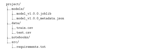

27.8 Complete Pipeline Example

Implementation Notes

End-to-End Pipeline with All Features:

from sklearn.pipeline import Pipeline
from sklearn.compose import ColumnTransformer
from sklearn.preprocessing import StandardScaler, OneHotEncoder
from sklearn.impute import SimpleImputer
from sklearn.ensemble import RandomForestClassifier
from sklearn.model_selection import cross_val_score
import pandas as pd
import joblib

# Define column types
numeric_features = ['age', 'income', 'credit_score']
categorical_features = ['gender', 'education', 'employment']

# Numeric pipeline
numeric_transformer = Pipeline([
    ('imputer', SimpleImputer(strategy='median')),
    ('scaler', StandardScaler())
])

# Categorical pipeline
categorical_transformer = Pipeline([
    ('imputer', SimpleImputer(strategy='most_frequent')),
    ('onehot', OneHotEncoder(handle_unknown='ignore'))
])

# Combine with ColumnTransformer
preprocessor = ColumnTransformer([
    ('num', numeric_transformer, numeric_features),
    ('cat', categorical_transformer, categorical_features)
])

# Full pipeline
pipeline = Pipeline([
    ('preprocessor', preprocessor),
    ('classifier', RandomForestClassifier(random_state=42))
])

# Cross-validation
cv_scores = cross_val_score(
    pipeline, X_train, y_train, 
    cv=5, scoring='accuracy'
)
print(f"CV Accuracy: {cv_scores.mean():.3f} (+/- {cv_scores.std():.3f})")

# Train final model
pipeline.fit(X_train, y_train)

# Evaluate
test_score = pipeline.score(X_test, y_test)
print(f"Test Accuracy: {test_score:.3f}")

# Save
joblib.dump(pipeline, 'credit_model_pipeline.joblib')

# Later: Load and predict
loaded_pipeline = joblib.load('credit_model_pipeline.joblib')
new_predictions = loaded_pipeline.predict(X_new)

28 Model Deployment

28.1 Deployment Considerations

Key Idea

Key Questions Before Deployment:

1. Latency Requirements:

• Real-time (\(<\) 100ms): Lightweight models, caching

• Near real-time (seconds): Most models acceptable

• Batch processing (hours): Any model size

2. Scale:

• Queries per second (QPS)?

• Peak vs average load?

• Need for horizontal scaling?

3. Infrastructure:

• Cloud (AWS, GCP, Azure) vs on-premise?

• Serverless (Lambda) vs containers (Docker) vs VMs?

• GPU required?

4. Monitoring:

• Performance metrics (latency, throughput)

• Model metrics (accuracy, drift detection)

• System metrics (CPU, memory, errors)

5. Updates:

• How often to retrain?

• Blue-green deployment vs canary?

• Rollback strategy?

28.2 Model Export Formats

28.2.1 ONNX (Open Neural Network Exchange)

Definition 28.1 (ONNX). ONNX is an open format for representing ML models, enabling interoperability across frameworks.

Benefits:

• Train in one framework (PyTorch, scikit-learn), deploy in another

• Optimized inference engines (ONNX Runtime)

• Hardware acceleration support

• Language-agnostic (use from Python, C++, Java, etc.)

# Convert scikit-learn to ONNX
from skl2onnx import convert_sklearn
from skl2onnx.common.data_types import FloatTensorType

# Define input type
initial_type = [('float_input', FloatTensorType([None, n_features]))]

# Convert
onnx_model = convert_sklearn(
    sklearn_model, 
    initial_types=initial_type
)

# Save
with open("model.onnx", "wb") as f:
    f.write(onnx_model.SerializeToString())

# Load and inference with ONNX Runtime
import onnxruntime as rt

sess = rt.InferenceSession("model.onnx")
input_name = sess.get_inputs()[0].name
pred = sess.run(None, {input_name: X_test.astype(np.float32)})

28.2.2 TensorFlow SavedModel

Definition 28.2 (TensorFlow SavedModel). TensorFlow’s universal format for saving models.

import tensorflow as tf

# Save
model.save('saved_model/my_model')

# Load
loaded_model = tf.keras.models.load_model('saved_model/my_model')

# Predict
predictions = loaded_model.predict(X_test)

Benefits:

• Complete model serialization (architecture + weights + config)

• TensorFlow Serving integration

• TensorFlow Lite for mobile/edge

28.2.3 Format Comparison

Model export format comparison

Format	Framework	Use Case	Pros
Pickle/Joblib	Any Python	Python-only	Simple, native
ONNX	Cross-framework	Production	Optimized, portable
SavedModel	TensorFlow	TF ecosystem	Complete, TF Serving
PMML	Traditional ML	Enterprise	Standardized, legacy

28.3 Serving Models via REST API

28.3.1 Flask API

Implementation Notes

Simple Flask API for Model Serving:

from flask import Flask, request, jsonify
import joblib
import numpy as np

# Initialize Flask app
app = Flask(__name__)

# Load model at startup
model = joblib.load('model_pipeline.joblib')

@app.route('/predict', methods=['POST'])
def predict():
    try:
        # Get JSON data
        data = request.get_json()
        
        # Convert to array
        features = np.array(data['features']).reshape(1, -1)
        
        # Predict
        prediction = model.predict(features)
        probability = model.predict_proba(features)
        
        # Return response
        return jsonify({
            'prediction': int(prediction[0]),
            'probability': probability[0].tolist(),
            'status': 'success'
        })
    
    except Exception as e:
        return jsonify({
            'error': str(e),
            'status': 'error'
        }), 400

@app.route('/health', methods=['GET'])
def health():
    return jsonify({'status': 'healthy'})

if __name__ == '__main__':
    app.run(host='0.0.0.0', port=5000)

Test with curl:

curl -X POST http://localhost:5000/predict \
  -H "Content-Type: application/json" \
  -d '{"features": [25, 50000, 700, 1, 2]}'

28.3.2 FastAPI (Modern Alternative)

Implementation Notes

FastAPI for High-Performance Serving:

from fastapi import FastAPI, HTTPException
from pydantic import BaseModel
import joblib
import numpy as np

# Define input schema
class PredictionRequest(BaseModel):
    features: list[float]

class PredictionResponse(BaseModel):
    prediction: int
    probability: list[float]

# Initialize app
app = FastAPI(title="ML Model API")

# Load model
model = joblib.load('model_pipeline.joblib')

@app.post("/predict", response_model=PredictionResponse)
async def predict(request: PredictionRequest):
    try:
        features = np.array(request.features).reshape(1, -1)
        prediction = model.predict(features)
        probability = model.predict_proba(features)
        
        return PredictionResponse(
            prediction=int(prediction[0]),
            probability=probability[0].tolist()
        )
    except Exception as e:
        raise HTTPException(status_code=400, detail=str(e))

@app.get("/health")
async def health():
    return {"status": "healthy"}

# Run with: uvicorn main:app --reload

FastAPI Advantages:

• Automatic API documentation (Swagger UI at /docs)

• Type validation with Pydantic

• Async support (higher throughput)

• Modern, faster than Flask

28.4 Containerization with Docker

Implementation Notes

Dockerfile for ML API:

FROM python:3.9-slim

WORKDIR /app

# Copy requirements and install
COPY requirements.txt .
RUN pip install --no-cache-dir -r requirements.txt

# Copy model and code
COPY model_pipeline.joblib .
COPY app.py .

# Expose port
EXPOSE 5000

# Run app
CMD ["python", "app.py"]

Build and Run:

# Build image
docker build -t ml-model-api .

# Run container
docker run -p 5000:5000 ml-model-api

# Test
curl http://localhost:5000/health

Docker Compose for Multi-Service:

version: '3.8'

services:
  api:
    build: .
    ports:
      - "5000:5000"
    environment:
      - MODEL_PATH=/models/model.joblib
    volumes:
      - ./models:/models
  
  redis:
    image: redis:alpine
    ports:
      - "6379:6379"

28.5 Cloud Deployment

Key Idea

Cloud Deployment Options:

1. Serverless (AWS Lambda, Google Cloud Functions):

• Pros: No server management, auto-scaling, pay per use

• Cons: Cold starts, limited execution time, limited memory

• Best for: Low to medium traffic, event-driven, cost-sensitive

2. Containers (AWS ECS, GKE, Azure Container Instances):

• Pros: Consistent environments, easy scaling, orchestration

• Cons: More complex setup, need to manage infrastructure

• Best for: Medium to high traffic, microservices

3. Managed ML Services:

• AWS SageMaker, Google AI Platform, Azure ML

• Pros: Built-in monitoring, auto-scaling, A/B testing, versioning

• Cons: Vendor lock-in, can be expensive

• Best for: Enterprise ML, need full MLOps

4. Kubernetes:

• Pros: Highly scalable, flexible, cloud-agnostic

• Cons: Steep learning curve, operational overhead

• Best for: Large scale, multi-model serving, complex workflows

28.6 Model Monitoring

Definition 28.3 (Model Monitoring). Continuous tracking of model performance and data quality in production.

Key Metrics to Monitor:

1. Performance Metrics:

• Prediction accuracy/error

• Latency (p50, p95, p99)

• Throughput (requests per second)

2. Data Quality:

• Missing values

• Out-of-range values

• Data type mismatches

3. Data Drift:

• Feature distribution changes

• Target distribution changes

• KL divergence, KS test

4. Concept Drift:

• \(P(y|X)\) changes over time

• Model accuracy degrades

• Need retraining

5. System Metrics:

• CPU/memory usage

• Error rates

• Uptime

Implementation Notes

Simple Logging for Monitoring:

import logging
import time
from datetime import datetime

# Setup logging
logging.basicConfig(level=logging.INFO)
logger = logging.getLogger(__name__)

@app.route('/predict', methods=['POST'])
def predict():
    start_time = time.time()
    
    try:
        data = request.get_json()
        features = np.array(data['features']).reshape(1, -1)
        
        # Predict
        prediction = model.predict(features)
        probability = model.predict_proba(features)
        
        # Log prediction
        latency = time.time() - start_time
        logger.info({
            'timestamp': datetime.now().isoformat(),
            'features': features.tolist(),
            'prediction': int(prediction[0]),
            'confidence': float(probability[0].max()),
            'latency_ms': latency * 1000
        })
        
        return jsonify({
            'prediction': int(prediction[0]),
            'probability': probability[0].tolist()
        })
    
    except Exception as e:
        logger.error(f"Prediction error: {str(e)}")
        return jsonify({'error': str(e)}), 400

Advanced: Use dedicated tools like Prometheus, Grafana, ELK stack, or cloud-native solutions (CloudWatch, Stackdriver).

28.7 Best Practices Summary

1. Versioning: Tag models, save metadata, track lineage

2. Testing: Unit tests, integration tests, load tests before production

3. Monitoring: Log predictions, track performance, detect drift

4. Gradual Rollout: Canary deployment (5% \(\to\) 50% \(\to\) 100%)

5. Rollback Plan: Keep previous model version, quick rollback capability

6. Security:

   • API authentication (API keys, OAuth)

   • Rate limiting

   • Input validation

   • HTTPS only

7. Documentation: API docs, model cards, usage examples

8. Automation: CI/CD pipeline for model updates

9. Cost Optimization: Right-size resources, use caching, batch predictions when possible

10. Feedback Loop: Collect ground truth labels, retrain periodically

28.8 Summary of Part 7

1. WEKA: GUI-based tool excellent for learning and quick experiments. Good for prototyping but not production. Easy algorithm comparison.

2. Scikit-learn Pipelines: Chain preprocessing and modeling. Prevents data leakage, enables hyperparameter tuning on entire workflow. Use ColumnTransformer for mixed data types.

3. Model Persistence: Use joblib for scikit-learn models. Save metadata (version, hyperparameters, performance). Version control models.

4. Export Formats: ONNX for cross-framework compatibility, SavedModel for TensorFlow ecosystem, pickle/joblib for Python-only.

5. API Serving: Flask for simple APIs, FastAPI for high performance. Include health checks and error handling.

6. Containerization: Docker ensures consistent environments. Docker Compose for multi-service setups.

7. Cloud Deployment: Choose based on scale (serverless \(\to\) containers \(\to\) Kubernetes). Managed services for full MLOps.

8. Monitoring: Track performance, data drift, system metrics. Log predictions for debugging and retraining.

Next Steps: Part 8 covers advanced topics: reinforcement learning, representation learning, ethics in ML, and modern trends like foundation models and AutoML.

Exercise 28.4.

1. Design a WEKA workflow to compare Decision Tree (J48), Random Forest, and SVM on the Iris dataset. What test method would you use and why?

2. Create a scikit-learn pipeline that handles both numeric (scaling) and categorical (one-hot encoding) features, then trains a Random Forest. Include proper error handling.

3. Explain why we must fit transformers only on training data. Give an example of what goes wrong if we fit on test data.

4. Design a Flask API that serves a sentiment analysis model. Include endpoints for single prediction and batch prediction. Add appropriate error handling.

5. Write a Dockerfile for deploying a scikit-learn model as a Flask API. What base image would you use? Why?

6. Compare serverless (AWS Lambda) vs container (Docker on ECS) deployment for: (a) Low-traffic app (100 requests/day), (b) High-traffic app (10,000 requests/second).

7. Design a monitoring system for a production model. What metrics would you track? How would you detect when the model needs retraining?

8. Implement a simple A/B test framework where 10% of traffic goes to a new model version, 90% to the old version. How would you decide when to fully switch?

Part 8: Advanced Topics and Modern Directions

29 Reinforcement Learning

29.1 Introduction to Reinforcement Learning

Definition 29.1 (Reinforcement Learning). Reinforcement Learning (RL) is learning by interacting with an environment to maximize cumulative reward.

Key difference from supervised learning:

• No labeled examples—agent must discover good actions through trial and error

• Delayed rewards—actions may have long-term consequences

• Sequential decision-making—current action affects future states

29.2 Core Components

Definition 29.2 (RL Framework). An RL system consists of:

1. Agent: The learner/decision maker

2. Environment: Everything the agent interacts with

3. State (\(s_t\)): Current situation of the agent

4. Action (\(a_t\)): Choice made by the agent

5. Reward (\(r_t\)): Immediate feedback from environment

6. Policy (\(\pi\)): Agent’s strategy for selecting actions \[\pi(a|s) = P(\text{action } a | \text{state } s)\]

7. Value Function (\(V^\pi(s)\)): Expected cumulative reward from state \(s\) under policy \(\pi\) \[V^\pi(s) = \mathbb{E}_\pi\left[\sum_{t=0}^\infty \gamma^t r_t \mid s_0 = s\right]\] where \(\gamma \in [0, 1]\) is the discount factor.

8. Q-Function (\(Q^\pi(s,a)\)): Expected cumulative reward from taking action \(a\) in state \(s\) \[Q^\pi(s,a) = \mathbb{E}_\pi\left[\sum_{t=0}^\infty \gamma^t r_t \mid s_0 = s, a_0 = a\right]\]

Agent-Environment interaction in RL

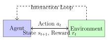
Intuition 256. Think of learning to play a video game:

• State: Current game screen

• Action: Button presses (up, down, left, right, jump)

• Reward: Points gained, lives lost

• Policy: Strategy for playing (e.g., “when enemy approaches, jump”)

• Goal: Maximize total score (cumulative reward)

The agent explores different actions, observes rewards, and learns which actions lead to high scores.

29.3 The Exploration-Exploitation Dilemma

Definition 29.4 (Exploration vs Exploitation). Exploitation: Choose the best-known action (maximize immediate reward)

Exploration: Try new actions to discover potentially better options

Dilemma: How to balance?

• Pure exploitation: May miss better strategies

• Pure exploration: Wastes time on known bad actions

\(\epsilon\)-Greedy Strategy: \[a_t = \begin{cases} \mathop{\mathrm{arg\,max}}_a Q(s_t, a) & \text{with probability } 1-\epsilon \text{ (exploit)} \\ \text{random action} & \text{with probability } \epsilon \text{ (explore)} \end{cases}\] Common: Start with high \(\epsilon\) (e.g., 1.0), decay over time to 0.01.

29.4 Q-Learning

Definition 29.5 (Q-Learning). Model-free algorithm to learn optimal Q-function (and thus optimal policy).

Bellman Optimality Equation: \[Q^*(s,a) = \mathbb{E}_{s' \sim P(\cdot|s,a)}\left[r(s,a) + \gamma \max_{a'} Q^*(s', a')\right]\] The optimal Q-value equals expected immediate reward plus discounted max future Q-value. In deterministic environments, this simplifies to \(Q^*(s,a) = r + \gamma \max_{a'} Q^*(s', a')\).

Q-Learning Update Rule: \[Q(s_t, a_t) \leftarrow Q(s_t, a_t) + \alpha\left[r_t + \gamma \max_{a} Q(s_{t+1}, a) - Q(s_t, a_t)\right]\] where \(\alpha\) is the learning rate.

Intuition: Adjust Q-value toward the observed return (TD error).

Algorithm Summary

Q-Learning Algorithm

Initialize: Q-table \(Q(s,a) = 0\) for all states \(s\) and actions \(a\)

For each episode:

1. Initialize state \(s\)

2. While not terminal:

   • Choose action \(a\) using \(\epsilon\)-greedy policy based on \(Q(s, \cdot)\)

   • Take action \(a\), observe reward \(r\) and next state \(s'\)

   • Update: \[Q(s,a) \leftarrow Q(s,a) + \alpha\left[r + \gamma \max_{a'} Q(s',a') - Q(s,a)\right]\]

   • \(s \leftarrow s'\)

Output: Learned Q-table, optimal policy \(\pi^*(s) = \mathop{\mathrm{arg\,max}}_a Q(s,a)\)

Example 29.6 (GridWorld Navigation). Agent in \(4 \times 4\) grid, goal at top-right corner.

States: Grid positions Actions: \(\{\text{up, down, left, right}\}\) Rewards: \(-1\) per step, \(+10\) at goal, \(-10\) for obstacles

Q-learning discovers shortest path by learning Q-values for each (state, action) pair.

29.5 Deep Q-Networks (DQN)

Definition 29.7 (DQN). Extend Q-learning to high-dimensional state spaces (e.g., images) using neural networks.

Instead of Q-table, use neural network \(Q(s, a; \theta)\) parameterized by \(\theta\).

Key innovations:

1. Experience Replay:

• Store transitions \((s_t, a_t, r_t, s_{t+1})\) in replay buffer

• Sample random mini-batches for training

• Breaks correlation between consecutive samples

2. Target Network:

• Use separate network \(Q(s, a; \theta^-)\) for target computation

• Update \(\theta^-\) periodically (copy from \(\theta\))

• Stabilizes training (target doesn’t move every update)

Loss Function: \[\mathcal{L}(\theta) = \mathbb{E}_{(s,a,r,s') \sim \text{Buffer}}\left[\left(r + \gamma \max_{a'} Q(s', a'; \theta^-) - Q(s, a; \theta)\right)^2\right]\]

Key Idea

DQN Breakthroughs:

Success: DQN (2013-2015) achieved human-level performance on Atari games using only pixel input.

Why important:

• First deep RL success on complex tasks

• Showed RL can work with raw sensory input

• Sparked modern deep RL research

Extensions:

• Double DQN: Addresses overestimation bias

• Dueling DQN: Separate value and advantage streams

• Prioritized Experience Replay: Sample important transitions more

• Rainbow: Combines multiple improvements

Limitations:

• Sample inefficient (needs millions of frames)

• Discrete actions only

• Can be unstable

29.6 Policy Gradient Methods

Definition 29.8 (Policy Gradient). Instead of learning Q-function, directly learn policy \(\pi(a|s; \theta)\).

Objective: Maximize expected cumulative reward \[J(\theta) = \mathbb{E}_{\tau \sim \pi_\theta}\left[\sum_t r_t\right]\]

Policy Gradient Theorem: \[\nabla_\theta J(\theta) = \mathbb{E}_{\tau \sim \pi_\theta}\left[\sum_t \nabla_\theta \log \pi_\theta(a_t|s_t) \cdot G_t\right]\] where \(G_t = \sum_{k=t}^\infty \gamma^{k-t} r_k\) is return from time \(t\).

Intuition: Increase probability of actions that led to high returns.

Modern Algorithms:

• REINFORCE: Basic policy gradient

• Actor-Critic: Combines policy gradient with value function

• A3C: Asynchronous actor-critic

• PPO (Proximal Policy Optimization): State-of-the-art, stable

• SAC (Soft Actor-Critic): Maximum entropy RL

29.7 Applications of RL

• Game Playing: AlphaGo, OpenAI Five (Dota 2), AlphaStar (StarCraft)

• Robotics: Manipulation, locomotion, drone control

• Autonomous Vehicles: Path planning, decision making

• Recommendation Systems: Sequential recommendations

• Resource Management: Data center cooling, traffic light control

• Finance: Trading, portfolio management

• Healthcare: Treatment optimization, drug dosing

30 Representation Learning

30.1 Introduction to Representation Learning

Definition 30.1 (Representation Learning). Learning good representations (features) of data automatically, rather than hand-crafting them.

Goal: Discover abstractions that make it easier to extract useful information for downstream tasks.

Good representations:

• Capture relevant factors of variation

• Disentangle underlying causes

• Robust to noise

• Transfer across tasks

30.2 Autoencoders

Definition 30.2 (Autoencoder). Neural network trained to reconstruct its input through a bottleneck.

Architecture:

• Encoder: \(\boldsymbol{z} = f_{\text{enc}}(\boldsymbol{x})\) (compress to latent code)

• Decoder: \(\hat{\boldsymbol{x}} = f_{\text{dec}}(\boldsymbol{z})\) (reconstruct)

Training: Minimize reconstruction error \[\mathcal{L}= \frac{1}{n}\sum_{i=1}^n \left\lVert\boldsymbol{x}_i - \hat{\boldsymbol{x}}_i\right\rVert^2\]

The bottleneck forces the network to learn compressed, meaningful representations.

Autoencoder architecture: compression and reconstruction

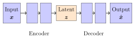
30.2.1 Variants of Autoencoders

Definition 30.3 (Autoencoder Variants). 1. Denoising Autoencoder (DAE):

• Input: Corrupted version \(\tilde{\boldsymbol{x}}\) (add noise)

• Target: Original clean \(\boldsymbol{x}\)

• Forces learning robust features

2. Sparse Autoencoder:

• Add sparsity penalty: \(\mathcal{L}= \text{reconstruction} + \lambda \sum_j |z_j|\)

• Encourages few active latent units

3. Variational Autoencoder (VAE):

• Learns probability distribution \(p(\boldsymbol{z}|\boldsymbol{x})\)

• Encoder outputs \(\mu\) and \(\sigma\) of Gaussian

• Can generate new samples by sampling from \(p(\boldsymbol{z})\)

• Loss: \(\mathcal{L}= \text{reconstruction} + \text{KL}(q(\boldsymbol{z}|\boldsymbol{x}) \| p(\boldsymbol{z}))\)

4. Contractive Autoencoder:

• Penalizes sensitivity of encoding to input perturbations

• More robust representations

Key Idea

Applications of Autoencoders:

• Dimensionality reduction: Alternative to PCA (non-linear)

• Anomaly detection: High reconstruction error \(\to\) anomaly

• Denoising: Remove noise from images, audio

• Data generation: VAEs generate new samples

• Feature learning: Use latent codes as features for downstream tasks

• Pretraining: Initialize networks for supervised learning

30.3 Word Embeddings

30.3.1 Motivation

Definition 30.4 (Word Representation Problem). How to represent words for machine learning?

One-hot encoding: \[\text{``cat''} = [0, 0, 1, 0, \ldots, 0], \quad \text{``dog''} = [0, 0, 0, 1, \ldots, 0]\]

Problems:

• High-dimensional (\(|V|\) for vocabulary size)

• Sparse (only one 1)

• No semantic similarity (all words equally distant)

Solution: Dense, low-dimensional embeddings that capture semantics.

30.3.2 Word2Vec

Definition 30.5 (Word2Vec). Learn word embeddings by predicting context words.

Two architectures:

1. CBOW (Continuous Bag of Words):

• Input: Context words

• Output: Target (center) word

• Predict word from its context

2. Skip-gram:

• Input: Target word

• Output: Context words

• Predict context from word

Training objective (Skip-gram): \[\max \frac{1}{T}\sum_{t=1}^T \sum_{-c \leq j \leq c, j \neq 0} \log P(w_{t+j} | w_t)\] where \(c\) is context window size.

Probability: \[P(w_O | w_I) = \frac{\exp(\boldsymbol{v}_{w_O}^\top \boldsymbol{v}_{w_I})}{\sum_{w \in V} \exp(\boldsymbol{v}_w^\top \boldsymbol{v}_{w_I})}\]

Key Idea

Word2Vec Properties:

Semantic similarity:

• Similar words have similar embeddings

• \(\text{similarity}(\text{``cat''}, \text{``dog''}) > \text{similarity}(\text{``cat''}, \text{``car''})\)

Analogies: \[\boldsymbol{v}_{\text{king}} - \boldsymbol{v}_{\text{man}} + \boldsymbol{v}_{\text{woman}} \approx \boldsymbol{v}_{\text{queen}}\] Vector arithmetic captures relationships!

Composition:

• “New York” = embedding of “New” + embedding of “York”

Training efficiency:

• Negative sampling: Instead of full softmax over \(|V|\), sample few negative examples

• Hierarchical softmax: Use tree structure for faster computation

30.3.3 GloVe

Definition 30.6 (GloVe (Global Vectors)). Learn embeddings by factorizing word co-occurrence matrix.

Objective: \[J = \sum_{i,j=1}^{|V|} f(X_{ij})(\boldsymbol{w}_i^\top \tilde{\boldsymbol{w}}_j + b_i + \tilde{b}_j - \log X_{ij})^2\] where:

• \(X_{ij}\): Number of times word \(j\) appears in context of word \(i\)

• \(f(X_{ij})\): Weighting function (down-weight rare co-occurrences)

Advantage: Uses global corpus statistics (Word2Vec uses local context).

30.4 Contrastive Learning

Definition 30.7 (Contrastive Learning). Learn representations by contrasting similar and dissimilar examples.

Core idea: Pull similar examples together, push dissimilar ones apart in embedding space.

SimCLR (Simple Framework for Contrastive Learning):

1. Data augmentation: Create two views of each image (crop, color jitter, etc.)

2. Encode: Pass through neural network \(f(\cdot)\) to get embeddings

3. Project: Apply projection head \(g(\cdot)\) to get \(\boldsymbol{z}\)

4. Contrastive loss: \[\ell_{i,j} = -\log \frac{\exp(\text{sim}(\boldsymbol{z}_i, \boldsymbol{z}_j)/\tau)}{\sum_{k=1}^{2N} \mathbb{1}_{k \neq i} \exp(\text{sim}(\boldsymbol{z}_i, \boldsymbol{z}_k)/\tau)}\] where \(\text{sim}(\boldsymbol{u}, \boldsymbol{v}) = \boldsymbol{u}^\top\boldsymbol{v} / (\left\lVert\boldsymbol{u}\right\rVert\left\lVert\boldsymbol{v}\right\rVert)\) (cosine similarity).

Key Idea

Why Contrastive Learning is Powerful:

Self-supervised: No labels needed! Use data augmentation to create positive pairs.

State-of-the-art results:

• SimCLR: Competitive with supervised learning on ImageNet

• MoCo (Momentum Contrast): Efficient contrastive learning

• CLIP: Contrastive learning for image-text pairs (foundation of DALL-E)

Applications:

• Image classification (pretrain on unlabeled data)

• Few-shot learning (good representations with few labels)

• Transfer learning (transfer to downstream tasks)

• Multi-modal learning (vision + language)

Recent methods:

• BYOL (Bootstrap Your Own Latent): No negative pairs needed

• SimSiam: Even simpler, still effective

• SwAV: Clustering-based contrastive learning

31 Ethics and Fairness in Machine Learning

31.1 Bias and Discrimination

Definition 31.1 (Types of Bias in ML). 1. Data Bias:

• Historical bias: Data reflects past discrimination

• Sampling bias: Training data not representative of population

• Measurement bias: Features measured differently for different groups

2. Algorithmic Bias:

• Model amplifies existing biases

• Optimization objective doesn’t account for fairness

3. Interaction Bias:

• Feedback loops: Biased predictions reinforce themselves

• Example: Predictive policing \(\to\) more arrests in certain areas \(\to\) model predicts more crime there

Example 31.2 (Real-World Bias Cases). 1. COMPAS (Recidivism Prediction):

• Predicted re-arrest risk for defendants

• ProPublica investigation: Biased against African Americans

• Higher false positive rate for Black defendants

2. Hiring Algorithms:

• Amazon scrapped ML hiring tool (2018)

• Trained on historical data (mostly male applicants)

• Penalized resumes with “women’s” (e.g., “women’s chess club”)

3. Facial Recognition:

• Lower accuracy for women and people of color

• Training data predominantly white males

• Real consequences: wrongful arrests

4. Credit Scoring:

• ML models for loan approval

• May discriminate based on proxy variables (zip code \(\to\) race)

31.2 Fairness Definitions

Definition 31.3 (Fairness Metrics). 1. Demographic Parity (Statistical Parity): \[P(\hat{Y} = 1 | A = 0) = P(\hat{Y} = 1 | A = 1)\] Equal positive prediction rates across groups \(A\) (e.g., race, gender).

2. Equalized Odds: \[P(\hat{Y} = 1 | Y = y, A = 0) = P(\hat{Y} = 1 | Y = y, A = 1) \quad \text{for } y \in \{0, 1\}\] Equal TPR and FPR across groups.

3. Equal Opportunity: \[P(\hat{Y} = 1 | Y = 1, A = 0) = P(\hat{Y} = 1 | Y = 1, A = 1)\] Equal TPR (recall) across groups. Subset of equalized odds.

4. Predictive Parity: \[P(Y = 1 | \hat{Y} = 1, A = 0) = P(Y = 1 | \hat{Y} = 1, A = 1)\] Equal precision across groups.

5. Individual Fairness: Similar individuals should receive similar predictions (harder to formalize).

Key Idea

Fairness Trade-offs:

Impossibility results: Cannot satisfy all fairness definitions simultaneously (except in trivial cases).

Accuracy vs Fairness: Often a trade-off

• Unconstrained model: Highest accuracy, may be unfair

• Fair model: Lower accuracy, satisfies fairness constraints

Which fairness metric to use?

• Depends on context and stakeholders

• Medical diagnosis: Equal opportunity (equal TPR)

• Advertising: Demographic parity

• Criminal justice: Combination of metrics

Mitigation strategies:

• Pre-processing: Transform data to remove bias

• In-processing: Add fairness constraints to training

• Post-processing: Adjust predictions to satisfy fairness

31.3 Explainable AI (XAI)

Definition 31.4 (Explainability). The ability to explain or present ML predictions in understandable terms to humans.

Why important?:

• Trust: Users need to trust model decisions

• Debugging: Understand why model fails

• Regulation: GDPR “right to explanation”

• Fairness: Detect and fix bias

• Safety: Critical applications (healthcare, autonomous vehicles)

31.3.1 LIME (Local Interpretable Model-agnostic Explanations)

Definition 31.5 (LIME). Explain individual predictions by approximating the model locally with an interpretable model.

Algorithm:

1. Select instance \(\boldsymbol{x}\) to explain

2. Perturb \(\boldsymbol{x}\) to create neighborhood samples

3. Get predictions from black-box model on perturbed samples

4. Fit simple interpretable model (e.g., linear regression) weighted by proximity to \(\boldsymbol{x}\)

5. Explain prediction using interpretable model’s coefficients

Intuition: Fit a simple model locally around the prediction to understand what features matter.

Example 31.6 (LIME for Image Classification). Model predicts “husky” for an image.

LIME highlights image regions:

• Green regions: Support prediction (dog’s face, fur)

• Red regions: Against prediction (background)

Reveals: Model uses dog features (good) or background snow (bad—spurious correlation)?

31.3.2 SHAP (SHapley Additive exPlanations)

Definition 31.7 (SHAP). Uses Shapley values from cooperative game theory to assign each feature an importance value for a prediction.

Shapley value: Fair distribution of “payout” (prediction) among “players” (features).

Properties:

• Local accuracy: Explanation matches prediction

• Consistency: If feature contributes more, importance increases

• Missingness: Feature not used \(\to\) zero importance

Computation: \[\phi_i = \sum_{S \subseteq F \setminus \{i\}} \frac{|S|!(|F|-|S|-1)!}{|F|!}[f(S \cup \{i\}) - f(S)]\] Average marginal contribution of feature \(i\) across all feature subsets.

Advantages over LIME:

• Theoretical foundation (game theory)

• Consistent across models

• Can aggregate for global explanations

Implementation Notes

Using SHAP in Python:

import shap

# Train model
model = RandomForestClassifier()
model.fit(X_train, y_train)

# Create explainer
explainer = shap.TreeExplainer(model)

# Compute SHAP values
shap_values = explainer.shap_values(X_test)

# Visualize
shap.summary_plot(shap_values, X_test)  # Global
shap.force_plot(explainer.expected_value, 
                shap_values[0], X_test.iloc[0])  # Local

31.3.3 Other Interpretability Methods

• Attention Mechanisms: In Transformers, attention weights show which input tokens are important

• Saliency Maps: Gradient-based methods for images (highlight important pixels)

• Partial Dependence Plots (PDP): Show relationship between feature and prediction

• Counterfactual Explanations: “What would need to change for different prediction?”

• Anchors: Find sufficient conditions for prediction (“If age > 50 AND income > 100K, then approve”)

31.4 Responsible AI Practices

1. Diverse Teams: Include diverse perspectives in development

2. Data Auditing: Check training data for bias, representativeness

3. Fairness Testing: Evaluate model across demographic groups

4. Transparency: Document data sources, model architecture, limitations

5. Human Oversight: Keep humans in the loop for critical decisions

6. Regular Audits: Monitor model performance and fairness in production

7. Right to Appeal: Allow users to contest automated decisions

8. Privacy: Protect user data, use privacy-preserving techniques (differential privacy, federated learning)

9. Impact Assessment: Consider societal impact before deployment

10. Continuous Learning: Stay updated on fairness research and regulations

32 Modern Trends

32.1 Transfer Learning and Fine-Tuning

Definition 32.1 (Transfer Learning). Use knowledge learned from one task (source) to improve learning on a different but related task (target).

Why transfer?

• Limited labeled data for target task

• Training from scratch is expensive

• Pretrained models capture general features

Typical workflow:

1. Pretrain: Train model on large dataset (e.g., ImageNet)

2. Transfer: Use pretrained weights as initialization

3. Fine-tune: Train on target task with small learning rate

Key Idea

Transfer Learning Strategies:

1. Feature Extraction (Frozen Pretrained Model):

• Freeze all pretrained layers

• Add new layers on top

• Train only new layers

• Fast, works when target data is small and similar to source

2. Fine-Tuning All Layers:

• Unfreeze all layers

• Train entire network with small learning rate

• Best performance, needs more target data

3. Fine-Tuning Top Layers Only:

• Freeze early layers (general features)

• Unfreeze later layers (task-specific features)

• Balance between feature extraction and full fine-tuning

Success stories:

• Computer Vision: ResNet, EfficientNet pretrained on ImageNet

• NLP: BERT, GPT pretrained on massive text corpora

• Speech: Wav2Vec2 pretrained on unlabeled audio

32.2 Foundation Models

Definition 32.2 (Foundation Models). Large-scale models trained on broad data that can be adapted to a wide range of downstream tasks.

Characteristics:

• Trained on massive diverse datasets (web-scale)

• Billions of parameters

• Emergent capabilities (not explicitly trained for)

• General-purpose (adapt to many tasks)

Paradigm shift: \[\text{Traditional: Task-specific data} \to \text{Task-specific model}\] \[\text{Foundation: General data} \to \text{Foundation model} \to \text{Many tasks}\]

32.2.1 BERT (Bidirectional Encoder Representations from Transformers)

Definition 32.3 (BERT). Pretrained Transformer encoder (2018, Google).

Pretraining tasks:

• Masked Language Modeling (MLM): Mask 15% of tokens, predict them \[\text{Input: } \text{The [MASK] is on the table}\] \[\text{Predict: } \text{cat}\]

• Next Sentence Prediction (NSP): Predict if sentence B follows sentence A

Impact:

• State-of-the-art on many NLP tasks

• Spawned many variants (RoBERTa, ALBERT, DistilBERT)

• Showed power of bidirectional context

32.2.2 GPT (Generative Pre-trained Transformer)

Definition 32.4 (GPT Family). Autoregressive Transformer decoders (OpenAI).

GPT-1 (2018): 117M parameters GPT-2 (2019): 1.5B parameters GPT-3 (2020): 175B parameters GPT-4 (2023): Estimated \(>\)1T parameters (multimodal)

Training: Predict next token given previous tokens \[P(w_t | w_1, \ldots, w_{t-1})\]

Key insight: Scale \(+\) next token prediction \(=\) emergent abilities

• Few-shot learning: Learn from few examples in prompt

• In-context learning: Adapt to task from prompt alone

• Chain-of-thought reasoning: Generate step-by-step solutions

Key Idea

GPT-3 Capabilities:

Zero-shot: No examples, just task description

Translate to French: Hello, how are you?
Output: Bonjour, comment allez-vous?

Few-shot: Provide examples in prompt

Q: What is 2+2? A: 4
Q: What is 5+3? A: 8
Q: What is 7+9? A: 16

Emergent abilities (not seen in smaller models):

• Arithmetic

• Code generation

• Common sense reasoning

• Instruction following

Limitations:

• Hallucinations (generates plausible but false information)

• Bias from training data

• No grounding in real world

• Expensive to run

32.3 Federated Learning

Definition 32.5 (Federated Learning). Train models across decentralized devices without sharing raw data.

Workflow:

1. Server sends global model to clients

2. Each client trains on local data

3. Clients send model updates (not data) to server

4. Server aggregates updates into global model

5. Repeat

Aggregation (FedAvg): \[\boldsymbol{w}_{t+1} = \sum_{k=1}^K \frac{n_k}{n} \boldsymbol{w}_k^{(t)}\] Weighted average of client models by data size.

Key Idea

Benefits of Federated Learning:

• Privacy: Data never leaves device

• Reduced latency: On-device inference

• Regulatory compliance: GDPR, HIPAA

• Bandwidth efficiency: Share models, not data

Challenges:

• Non-IID data: Each client has different distribution

• Communication cost: Many rounds needed

• Heterogeneous devices: Different compute power

• Privacy attacks: Model updates can leak information

Applications:

• Mobile keyboards (Gboard)

• Healthcare (multiple hospitals, can’t share patient data)

• Finance (banks collaborate without sharing data)

• IoT devices

Enhanced privacy:

• Differential privacy: Add noise to updates

• Secure aggregation: Encrypted updates

• Homomorphic encryption: Compute on encrypted data

32.4 AutoML (Automated Machine Learning)

Definition 32.6 (AutoML). Automate the end-to-end process of applying ML to real-world problems.

Components:

• Data preprocessing

• Feature engineering

• Model selection

• Hyperparameter optimization

• Architecture search (for neural networks)

• Ensemble construction

32.4.1 Neural Architecture Search (NAS)

Definition 32.7 (NAS). Automatically design neural network architectures.

Search space: Define possible architectures (layers, connections, operations)

Search strategy:

• Random search

• Reinforcement learning

• Evolutionary algorithms

• Gradient-based (DARTS)

Performance estimation:

• Train from scratch (expensive)

• Early stopping

• Weight sharing (ENAS)

• Performance prediction

Success: NAS-discovered architectures (EfficientNet, AmoebaNet) outperform hand-designed ones.

32.4.2 AutoML Tools

• Auto-sklearn: Automated scikit-learn pipeline

• TPOT: Genetic programming for pipeline optimization

• H2O AutoML: Automated model selection and ensembling

• Google Cloud AutoML: Managed AutoML service

• AutoKeras: NAS for Keras

• PyCaret: Low-code ML library

Key Idea

AutoML: Democratization or Threat?

Pros:

• Lowers barrier to entry (non-experts can use ML)

• Frees experts to focus on problem formulation

• Often finds better models than manual search

• Reproducible workflows

Cons:

• Can be slow (lots of trials)

• Black box (hard to understand choices)

• May not consider domain constraints

• Expensive (compute cost)

Reality: AutoML is a tool, not a replacement. ML expertise still needed for:

• Problem formulation

• Data quality assessment

• Interpreting results

• Debugging failures

• Ethical considerations

32.5 Future Directions

Key Idea

Emerging Trends and Open Problems:

1. Multimodal Learning:

• Models that understand multiple modalities (text, image, audio, video)

• CLIP, DALL-E, Flamingo, GPT-4

2. Continual Learning:

• Learn new tasks without forgetting old ones

• Overcome catastrophic forgetting

3. Few-Shot and Zero-Shot Learning:

• Learn from very few examples

• Generalize to unseen classes

4. Causal Machine Learning:

• Go beyond correlation to causation

• Robust to distribution shift

• Counterfactual reasoning

5. Energy-Efficient ML:

• Reduce environmental impact (training GPT-3: tons of CO2)

• Model compression, pruning, quantization

• Efficient architectures

6. Trustworthy AI:

• Robustness to adversarial attacks

• Uncertainty quantification

• Certified defenses

7. Human-AI Collaboration:

• AI as assistant, not replacement

• Interactive ML

• Human-in-the-loop systems

8. Quantum Machine Learning:

• Leverage quantum computers for ML

• Quantum neural networks

• Early stage, potential for exponential speedups

32.6 Conclusion

Machine Learning is a rapidly evolving field with profound impact on society. As practitioners, we must:

1. Master fundamentals: Strong foundation enables understanding new methods

2. Stay curious: New papers, techniques, applications emerge daily

3. Think critically: Not every problem needs ML; not every solution is ethical

4. Embrace uncertainty: Models are tools, not truth

5. Prioritize ethics: Consider impact on individuals and society

6. Collaborate: ML is interdisciplinary—work with domain experts

7. Keep learning: The field evolves faster than any textbook

The journey from mathematical foundations to modern foundation models is remarkable. Yet the most exciting developments are still ahead. Whether through scientific breakthroughs, ethical frameworks, or novel applications, the future of ML will be shaped by thoughtful practitioners who combine technical skill with wisdom.

Your role: Build systems that are not just intelligent, but beneficial.

Exercise 32.8.

1. Design a Q-learning agent for a simple grid world. Define states, actions, rewards, and write the Q-update rule.

2. Explain why experience replay and target networks are crucial for DQN stability. What problems do they solve?

3. Compare PCA (from Part 5) and autoencoders for dimensionality reduction. When would you prefer autoencoders?

4. Given Word2Vec embeddings, explain why \(\boldsymbol{v}_{\text{king}} - \boldsymbol{v}_{\text{man}} + \boldsymbol{v}_{\text{woman}} \approx \boldsymbol{v}_{\text{queen}}\) works. What does this reveal about the embedding space?

5. A facial recognition system has 99% accuracy but 5% false positive rate for one demographic group vs 1% for another. Which fairness definition is violated? Propose a mitigation strategy.

6. You have 100 labeled examples and 10,000 unlabeled examples for image classification. Design a strategy using transfer learning and/or contrastive learning.

7. Compare fine-tuning BERT for sentiment analysis vs training a CNN from scratch. What are the trade-offs?

8. Design a federated learning system for predicting disease from hospital data. Address: communication efficiency, privacy, and non-IID data distributions.

End of Machine Learning Notes

“The best way to predict the future is to invent it.” — Alan Kay